Intro to Assembly Language

Cheat Sheet

Registers

Description	64-bit Register (8-bytes)	8-bit Register (1-bytes)
Data/Arguments Registers
Syscall Number/Return value	rax	al
Callee Saved	rbx	bl
1st arg	rdi	dil
2nd arg	rsi	sil
3rd arg	rdx	dl
4th arg - Loop Counter	rcx	cl
5th arg	r8	r8b
6th arg	r9	r9b
Pointer Registers
Base Stack Pointer	rbp	bpl
Current/Top Stack Pointer	rsp	spl
Instruction Pointer 'call only'	rip	ipl

Assembly and Disassembly

Command	Description
nasm -f elf64 helloWorld.s	Assemble code
ld -o helloWorld helloWorld.o	Link code
ld -o fib fib.o -lc --dynamic-linker /lib64/ld-linux-x86-64.so.2	Link code with libc functions
objdump -M intel -d helloWorld	Disassemble .text section
objdump -M intel --no-show-raw-insn --no-addresses -d helloWorld	Show binary assembly code
objdump -sj .data helloWorld	Disassemble .data section

GDB

Command	Description
gdb -q ./helloWorld	Open binary in gdb
info functions	View binary functions
info variables	View binary variables
registers	View registers
disas _start	Disassemble label/function
b _start	Break label/function
b *0x401000	Break address
r	Run the binary
x/4xg $rip	Examine register "x/ count-format-size $register"
si	Step to the next instruction
s	Step to the next line of code
ni	Step to the next function
c	Continue to the next break point
patch string 0x402000 "Patched!\\x0a"	Patch address value
set $rdx=0x9	Set register value

Assembly Instructions

Instruction	Description	Example
Data Movement
mov	Move data or load immediate data	mov rax, 1 -> rax = 1
lea	Load an address pointing to the value	lea rax, [rsp+5] -> rax = rsp+5
xchg	Swap data between two registers or addresses	xchg rax, rbx -> rax = rbx, rbx = rax
Unary Arithmetic Instructions
inc	Increment by 1	inc rax -> rax++ or rax += 1 -> rax = 2
dec	Decrement by 1	dec rax -> rax-- or rax -= 1 -> rax = 0
Binary Arithmetic Instructions
add	Add both operands	add rax, rbx -> rax = 1 + 1 -> 2
sub	Subtract Source from Destination (i.e rax = rax - rbx)	sub rax, rbx -> rax = 1 - 1 -> 0
imul	Multiply both operands	imul rax, rbx -> rax = 1 * 1 -> 1
Bitwise Arithmetic Instructions
not	Bitwise NOT (invert all bits, 0->1 and 1->0)	not rax -> NOT 00000001 -> 11111110
and	Bitwise AND (if both bits are 1 -> 1, if bits are different -> 0)	and rax, rbx -> 00000001 AND 00000010 -> 00000000
or	Bitwise OR (if either bit is 1 -> 1, if both are 0 -> 0)	or rax, rbx -> 00000001 OR 00000010 -> 00000011
xor	Bitwise XOR (if bits are the same -> 0, if bits are different -> 1)	xor rax, rbx -> 00000001 XOR 00000010 -> 00000011
Loops
mov rcx, x	Sets loop (rcx) counter to x	mov rcx, 3
loop	Jumps back to the start of loop until counter reaches 0	loop exampleLoop
Branching
jmp	Jumps to specified label, address, or location	jmp loop
jz	Destination equal to Zero	D = 0
jnz	Destination Not equal to Zero	D != 0
js	Destination is Negative	D < 0
jns	Destination is Not Negative (i.e. 0 or positive)	D >= 0
jg	Destination Greater than Source	D > S
jge	Destination Greater than or Equal Source	D >= S
jl	Destination Less than Source	D < S
jle	Destination Less than or Equal Source	D <= S
cmp	Sets RFLAGS by subtracting second operand from first operand (i.e. first - second)	cmp rax, rbx -> rax - rbx
Stack
push	Copies the specified register/address to the top of the stack	push rax
pop	Moves the item at the top of the stack to the specified register/address	pop rax
Functions
call	push the next instruction pointer rip to the stack, then jumps to the specified procedure	call printMessage
ret	pop the address at rsp into rip, then jump to it	ret

Functions

Command	Description
cat /usr/include/x86_64-linux-gnu/asm/unistd_64.h | grep write	Locate write syscall number
man -s 2 write	write syscall man page
man -s 3 printf	printf libc man page

Syscall Calling Convention

1. Save registers to stack
2. Set its syscall number in rax
3. Set its arguments in the registers
4. Use the syscall assembly instruction to call it

Function Calling Convention

1. Save Registers on the stack (Caller Saved)
2. Pass Function Arguments (like syscalls)
3. Fix Stack Alignment
4. Get Function's Return Value (in rax)

Shellcoding

Command	Description
pwn asm 'push rax' -c 'amd64'	Instruction to shellcode
pwn disasm '50' -c 'amd64'	Shellcode to instructions
python3 shellcoder.py helloworld	Extract binary shellcode
python3 loader.py '4831..0f05	Run shellcode
python assembler.py '4831..0f05	Assemble shellcode into binary
Shellcraft
pwn shellcraft -l 'amd64.linux'	List available syscalls
pwn shellcraft amd64.linux.sh	Generate syscalls shellcode
pwn shellcraft amd64.linux.sh -r	Run syscalls shellcode
Msfvenom
`msfvenom -l payloads \	grep 'linux/x64'`	List available syscalls
msfvenom -p 'linux/x64/exec' CMD='sh' -a 'x64' --platform 'linux' -f 'hex'	Generate syscalls shellcode
msfvenom -p 'linux/x64/exec' CMD='sh' -a 'x64' --platform 'linux' -f 'hex' -e 'x64/xor'	Generate encoded syscalls shellcode

Shellcoding Requirements

1. Does not contain variables
2. Does not refer to direct memory addresses
3. Does not contain any NULL bytes 00

---

Assembly Language

---

Most of our interaction with our personal computers and smartphones is done through the operating system and other applications. These applications are usually developed using high-level languages, like C++, Java, Python, and many others. We also know that each of these devices has a core processor that runs all of the necessary processes to execute systems and applications, along with Random Access Memory (RAM), Video Memory, and other similar components.

However, these physical components cannot interpret or understand high-level languages, as they can essentially only process 1's and 0's. This is where Assembly language comes in, as a low-level language that can write direct instructions the processors can understand. Since the processor can only process binary data "i.e. 1's and 0's", it would be challenging for humans to interact with processors without referring to manuals to know which hex code runs which instruction.

This is why low-level assembly languages were built. By using Assembly, developers can write human-readable machine instructions, which are then assembled into their machine code equivalent, so that the processor can directly run them. This is why some refer to Assembly language as symbolic machine code. For example, the Assembly code 'add rax, 1' is much more intuitive and easier to remember than its equivalent machine shellcode '4883C001', and easier to remember than the equivalent binary machine code '01001000 10000011 11000000 00000001'. As we can see, without Assembly language, it is very challenging to write machine instructions or directly interact with the processor.

Machine code is often represented as Shellcode, a hex representation of machine code bytes. Shellcode can be translated back to its Assembly counterpart and can also be loaded directly into memory as binary instructions to be executed.

---

High-level vs. Low-level

As there are different processor designs, each processor understands a different set of machine instructions and a different Assembly language. In the past, applications had to be written in assembly for each processor, so it was not easy to develop an application for multiple processors. In the early 1970's, high-level languages (like C) were developed to make it possible to write a single easy to understand code that can work on any processor without rewriting it for each processor. To be more specific, this was made possible by creating compilers for each language.

When high-level code is compiled, it is translated into assembly instructions for the processor it is being compiled for, which is then assembled into machine code to run on the processor. This is why compilers are built for various languages and various processors to convert the high-level code into assembly code and then machine code that matches the running processor.

Later on, interpreted languages were developed, like Python, PHP, Bash, JavaScript, and others, which are usually not compiled but are interpreted during run time. These types of languages utilize pre-built libraries to run their instructions. These libraries are typically written and compiled in other high-level languages like C or C++. So when we issue a command in an interpreted language, it would use the compiled library to run that command, which uses its assembly code/machine code to perform all the instructions necessary to run this command on the processor.

---

Compilation Stages

Let's take a basic 'Hello World!' program that prints these words on the screen and show how it changes from high-level to machine code. In an interpreted language, like Python, it would be the following basic line:

Code: python

print("Hello World!")

If we run this Python line, it would be essentially executing the following C code:

Code: c

#include <unistd.h>

int main()
{
    write(1, "Hello World!", 12);
    _exit(0);
}

Note: the actual C source code is much longer, but the above is the essence of how the string 'Hello World!' is printed. If you are ever interested in knowing more, you can check out the source code of the Python3 print function at this link and this link

The above C code uses the Linux write syscall, built-in for processes to write to the screen. The same syscall called in Assembly looks like the following:

Code: nasm

mov rax, 1
mov rdi, 1
mov rsi, message
mov rdx, 12
syscall

mov rax, 60
mov rdi, 0
syscall

As we can see, when the write syscall is called in C or Assembly, both are using 1, the text, and 12 as the arguments. This will be covered more in-depth later in the module. From this point, Assembly code, shellcode, and binary machine code are mostly identical but written in different formats. The previous Assembly code can be assembled into the following hex machine code (i.e., shellcode):

Code: shellcode

48 c7 c0 01
48 c7 c7 01
48 8b 34 25
48 c7 c2 0c
0f 05

48 c7 c0 3c
48 c7 c7 00
0f 05

Finally, for the processor to execute the instructions linked to this machine, it would have to be translated into binary, which would look like the following:

Code: binary

01001000 11000111 11000000 00000001
01001000 11000111 11000111 00000001
01001000 10001011 00110100 00100101
01001000 11000111 11000010 00001101 
00001111 00000101

01001000 11000111 11000000 00111100 
01001000 11000111 11000111 00000000 
00001111 00000101

A CPU uses different electrical charges for a 1 and a 0, and hence can calculate these instructions from the binary data once it receives them.

Note: With multi-platform languages, like Java, the code is compiled into a Java Bytecode, which is the same for all processors/systems, and is then compiled to machine code by the local Java Runtime environment. This is what makes Java relatively slower than other languages like C++ that compile directly into machine code. Languages like C++ are more suitable for processor intensive applications like games.

We now see how computer languages progressed from assembly language unique for each processor to high-level languages that can work on any device without even needing to be compiled.

---

Value for Pentesters

Understanding assembly language instructions is critical for binary exploitation, which is an essential part of penetration testing. When it comes to exploiting compiled programs, the only way to attack them would be through their binaries. To disassemble, debug, and follow binary instructions in memory and find potential vulnerabilities, we must have a basic understanding of Assembly language and how it flows through the CPU components.

This is why once we start learning binary exploitation techniques, like buffer overflows, ROP chains, heap exploitation, and others, we will be dealing a lot with assembly instructions and following them in memory. Furthermore, to exploit these vulnerabilities, we will have to build custom exploits that use assembly instructions to manipulate the code while in memory and inject assembly shellcode to be executed.

Learning Intel x86 Assembly Language is crucial for writing exploits for binaries on modern machines. In addition to Intel x86, ARM is becoming more common, as most modern smartphones and some modern laptops like the M1 MacBook Pro feature ARM processors. Exploiting binaries in these systems requires ARM Assembly knowledge. This module will not cover ARM Assembly Language. That being said, Assembly Language basics will undoubtedly be helpful to anyone willing to learn ARM Assembly since the two languages have a lot of similarities.

---

Computer Architecture

---

Today, most modern computers are built on what is known as the Von Neumann Architecture, which was developed back in 1945 by Von Neumann to enable the creation of "General-Purpose Computers" as Alan Turing described them at the time. Alan Turing in turn, based his ideas on Charles Babbage's mid-19th century "Programmable Computer" concept. Note that all of these people were mathematicians.

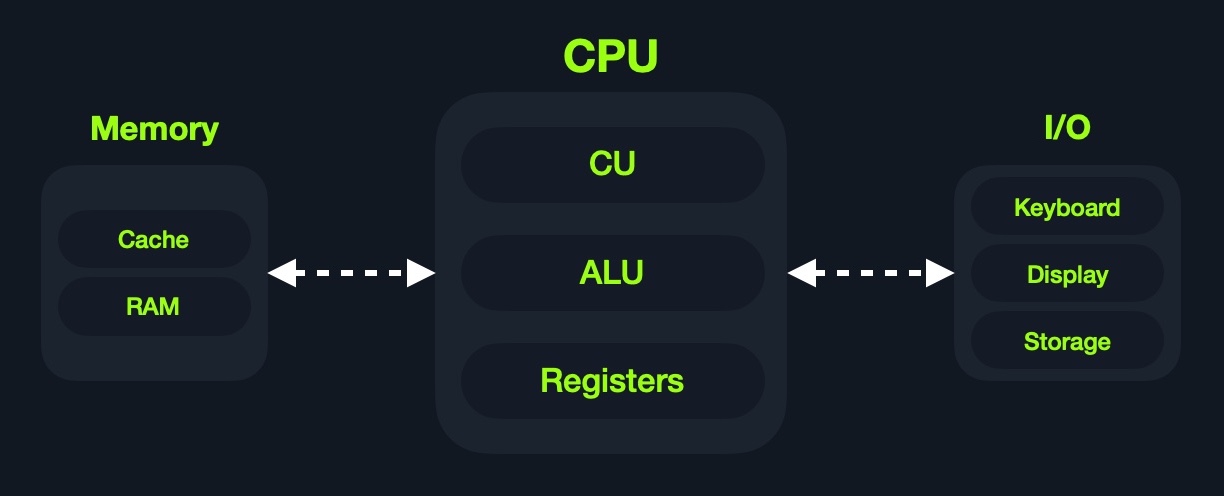
This architecture executes machine code to perform specific algorithms. It mainly consists of the following elements:

• Central Processing Unit (CPU)
• Memory Unit
• Input/Output Devices
  • Mass Storage Unit
  • Keyboard
  • Display

Furthermore, the CPU itself consists of three main components:

• Control Unit (CU)
• Arithmetic/Logic Unit (ALU)
• Registers

Though very old, this architecture is still the basis of most modern computers, servers, and even smartphones.

Assembly languages mainly work with the CPU and memory. This is why it is crucial to understand the general design of computer architecture, so when we start using assembly instructions to move and process data, we know where it's going and coming from and how fast/expensive each instruction is.

Furthermore, basic and advanced binary exploitation requires a proper understanding of computer architecture. With basic stack overflows, we only need to be aware of the general design. Once we start using ROP and Heap exploits, our understanding should be profound. Let us now take a deeper look into some essential components.

---

Memory

A computer's memory is where the temporary data and instructions of currently running programs are located. A computer's memory is also known as Primary Memory. It is the primary location the CPU uses to retrieve and process data. It does so very frequently (billions of times a second), so the memory must be extremely fast in storing and retrieving data and instructions.

There are two main types of memory:

1. Cache
2. Random Access Memory (RAM)

Cache

Cache memory is usually located within the CPU itself and hence is extremely fast compared to RAM, as it runs at the same clock speed as the CPU. However, it is very limited in size and very sophisticated, and expensive to manufacture due to it being so close to the CPU core.

Since RAM clock speed is usually much slower than the CPU cores, in addition to it being far from the CPU, if a CPU had to wait for the RAM to retrieve each instruction, it would effectively be running at much lower clock speeds. This is the main benefit of cache memory. It enables the CPU to access the upcoming instructions and data quicker than retrieving them from RAM.

There are usually three levels of cache memory, depending on their closeness to the CPU core:

Level	Description
Level 1 Cache	Usually in kilobytes, the fastest memory available, located in each CPU core. (Only registers are faster.)
Level 2 Cache	Usually in megabytes, extremely fast (but slower than L1), shared between all CPU cores.
Level 3 Cache	Usually in megabytes (larger than L2), faster than RAM but slower than L1/L2. (Not all CPUs use L3.)

RAM

RAM is much larger than cache memory, coming in sizes ranging from gigabytes up to terabytes. RAM is also located far away from the CPU cores and is much slower than cache memory. Accessing data from RAM addresses takes many more instructions.

For example, retrieving an instruction from the registers takes only one clock cycle, and retrieving it from the L1 cache takes a few cycles, while retrieving it from RAM takes around 200 cycles. When this is done billions of times a second, it makes a massive difference in the overall execution speed.

In the past, with 32-bit addresses, memory addresses were limited from 0x00000000 to 0xffffffff. This meant that the maximum possible RAM size was 2³² bytes, which is only 4 gigabytes, at which point we run out of unique addresses. With 64-bit addresses, the range is now up to 0xffffffffffffffff, with a theoretical maximum RAM size of 2⁶⁴ bytes, which is around 18.5 exabytes (18.5 million terabytes), so we shouldn't be running out of memory addresses anytime soon.

When a program is run, all of its data and instructions are moved from the storage unit to the RAM to be accessed when needed by the CPU. This happens because accessing them from the storage unit is much slower and will increase data processing times. When a program is closed, its data is removed or made available to re-use from the RAM.

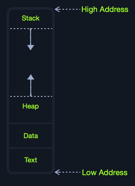
As we can see, the RAM is split into four main segments:

Segment	Description
Stack	Has a Last-in First-out (LIFO) design and is fixed in size. Data in it can only be accessed in a specific order by push-ing and pop-ing data.
Heap	Has a hierarchical design and is therefore much larger and more versatile in storing data, as data can be stored and retrieved in any order. However, this makes the heap slower than the Stack.
Data	Has two parts: Data, which is used to hold variables, and .bss, which is used to hold unassigned variables (i.e., buffer memory for later allocation).
Text	Main assembly instructions are loaded into this segment to be fetched and executed by the CPU.

Although this segmentation applies to the entire RAM, each application is allocated its Virtual Memory when it is run. This means that each application would have its own stack, heap, data, and text segments.

---

IO/Storage

Finally, we have the Input/Output devices, like the keyboard, the screen, or the long-term storage unit, also known as Secondary Memory. The processor can access and control IO devices using Bus Interfaces, which act as 'highways' to transfer data and addresses, using electrical charges for binary data.

Each Bus has a capacity of bits (or electrical charges) it can carry simultaneously. This usually is a multiple of 4-bits, ranging up to 128-bits. Bus interfaces are also usually used to access memory and other components outside the CPU itself. If we take a closer look at a CPU or a motherboard, we can see the bus interfaces all over them:

Unlike primary memory that is volatile and stores temporary data and instructions as the programs are running, the storage unit stores permanent data, like the operating system files or entire applications and their data.

The storage unit is the slowest to access. First, because they are the farthest away from the CPU, accessing them through bus interfaces like SATA or USB takes much longer to store and retrieve the data. They are also slower in their design to allow more data storage. Αs long as there is more data to go through, they will be slower.

There has been a shift from classic magnetic storage units, like tapes or Hard Disk Drives (HDD), to Solid-State Drives (SSD) in recent years. This is because SSD's utilize a similar design to RAM's, using non-volatile circuitry that retains data even without electricity. This made storage units much faster in storing and retrieving data. Still, since they are far away from the CPU and connected through special interfaces, they are the slowest unit to access.

---

Speed

As we can see from the above, the further away a component is from the CPU core, the slower it is. Also, the more data it can hold, the slower it is, as it simply has to go through more to fetch the data. The below table summarizes each component, its size, and its speed:

Component	Speed	Size
Registers	Fastest	Bytes
L1 Cache	Fastest, other than Registers	Kilobytes
L2 Cache	Very fast	Megabytes
L3 Cache	Fast, but slower than the above	Megabytes
RAM	Much slower than all of the above	Gigabytes-Terabytes
Storage	Slowest	Terabytes and more

The speed here is relative depending on the CPU clock speed. Now that we have a general idea of the computer architecture, we'll discuss Registers and the CPU architecture in the next section.

---

CPU Architecture

---

The Central Processing Unit (CPU) is the main processing unit within a computer. The CPU contains both the Control Unit (CU), which is in charge of moving and controlling data, and the Arithmetic/Logic Unit (ALU), which is in charge of performing various arithmetics and logical calculations as requested by a program through the assembly instructions.

The manner in which and how efficiently a CPU processes its instructions depends on its Instruction Set Architecture (ISA). There are multiple ISA's in the industry, each having its way of processing data. RISC architecture is based on processing more simple instructions, which takes more cycles, but each cycle is shorter and takes less power. The CISC architecture is based on fewer, more complex instructions, which can finish the requested instructions in fewer cycles, but each instruction takes more time and power to be processed.

Let us take a look at both RISC and CISC, and learn more about instructions cycles and registers.

---

Clock Speed & Clock Cycle

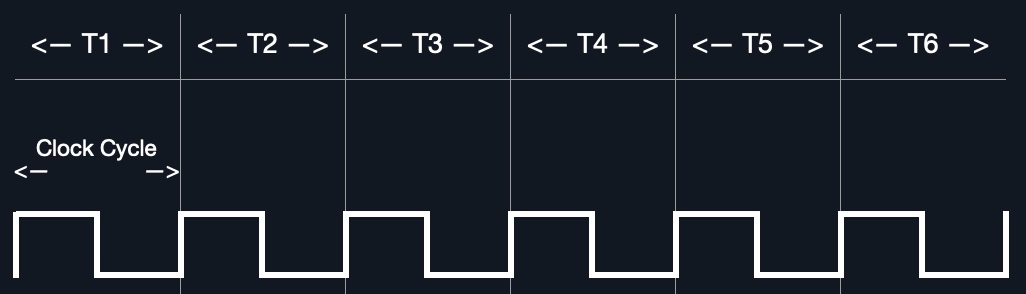
Each CPU has a clock speed that indicates its overall speed. Every tick of the clock runs a clock cycle that processes a basic instruction, such as fetching an address or storing an address. Specifically, this is done by the CU or ALU.

The frequency in which the cycles occur is counted is cycles per second (Hertz). If a CPU has a speed of 3.0 GHz, it can run 3 billion cycles every second (per core).

Modern processors have a multi-core design, allowing them to have multiple cycles at the same time.

---

Instruction Cycle

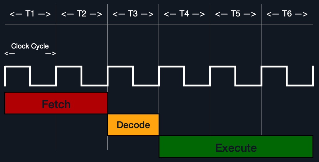
An Instruction Cycle is the cycle it takes the CPU to process a single machine instruction.

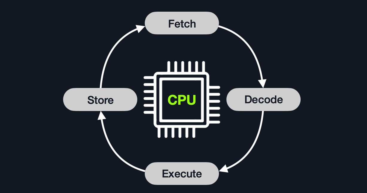
An instruction cycle consists of four stages: Fetch, Decode, Execute, and Store:

Instruction	Description
1. Fetch	Takes the next instruction's address from the Instruction Address Register (IAR), which tells it where the next instruction is located.
2. Decode	Takes the instruction from the IAR, and decodes it from binary to see what is required to be executed.
3. Execute	Fetch instruction operands from register/memory, and process the instruction in the ALU or CU.
4. Store	Store the new value in the destination operand.

All of the stages in the instruction cycle are carried out by the Control Unit, except when arithmetic instructions need to be executed "add, sub, ..etc", which are executed by the ALU.

Each Instruction Cycle takes multiple clock cycles to finish, depending on the CPU architecture and the complexity of the instruction. Once a single instruction cycle ends, the CU increments to the next instruction and runs the same cycle on it, and so on.

For example, if we were to execute the assembly instruction add rax, 1, it would run through an instruction cycle:

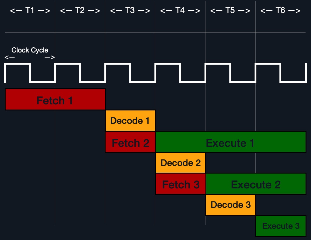
1. Fetch the instruction from the rip register, 48 83 C0 01 (in binary).
2. Decode '48 83 C0 01' to know it needs to perform an add of 1 to the value at rax.
3. Get the current value at rax (by CU), add 1 to it (by the ALU).
4. Store the new value back to rax.

In the past, processors used to process instructions sequentially, so they had to wait for one instruction to finish to start the next. On the other hand, modern processors can process multiple instructions in parallel by having multiple instruction/clock cycles running at the same time. This is made possible by having a multi-thread and multi-core design.

---

Processor Specific

As previously mentioned, each processor understands a different set of instructions. For example, while an Intel processor based on the 64-bit x86 architecture may interpret the machine code 4883C001 as add rax, 1, an ARM processor translates the same machine code as the biceq r8, r0, r8, asr #6 instruction. As we can see, the same machine code performs an entirely different instruction on each processor.

This is because each processor type has a different low-level assembly language architecture known as Instruction Set Architectures (ISA). For example, the add instruction seen above, add rax, 1 is for Intel x86 64-bit processors. The same instruction written for the ARM processor assembly language is represented as add r1, r1, 1.

It is important to understand that each processor has its own set of instructions and corresponding machine code.

Furthermore, a single Instruction Set Architecture may have several syntax interpretations for the same assembly code. For example, the above add instruction is based on the x86 architecture, which is supported by multiple processors like Intel, AMD, and legacy AT\&T processors. The instruction is written as add rax, 1 with Intel syntax, and written as addb $0x1,%rax with AT\&T syntax.

As we can see, even though we can tell that both instructions are similar and do the same thing, their syntax is different, and the locations of the source and destination operands are swapped as well. Still, both codes assemble the same machine code and perform the same instruction.

So, each processor type has its Instruction Set Architectures, and each architecture can be further represented in several syntax formats

This module will focus mainly on the Intel x86 64-bit assembly language (also known as x86_64 and AMD64), as the majority of modern computers and servers run on this processor architecture. We will be using the Intel syntax as well.

If we want to know whether our Linux system supports x86_64 architecture, we can use the lscpu command:

CPU Architecture

root@htb[/htb]$ lscpu

Architecture:                    x86_64
CPU op-mode(s):                  32-bit, 64-bit
Byte Order:                      Little Endian

<SNIP>

As we can see in the above output, the CPU architecture is x86_64, and supports 32-bit and 64-bit. The byte order is Little Endian. We can also use the uname -m command to get the CPU architecture. We will discuss the two most common Instruction Set Architectures in the next section: CISC and RISC.

---

Instruction Set Architectures

---

An Instruction Set Architecture (ISA) specifies the syntax and semantics of the assembly language on each architecture. It is not just a different syntax but is built in the core design of a processor, as it affects the way and order instructions are executed and their level of complexity. ISA mainly consists of the following components:

• Instructions
• Registers
• Memory Addresses
• Data Types

Component	Description	Example
Instructions	The instruction to be processed in the opcode operand_list format. There are usually 1,2, or 3 comma-separated operands.	add rax, 1, mov rsp, rax, push rax
Registers	Used to store operands, addresses, or instructions temporarily.	rax, rsp, rip
Memory Addresses	The address in which data or instructions are stored. May point to memory or registers.	0xffffffffaa8a25ff, 0x44d0, $rax
Data Types	The type of stored data.	byte, word, double word

These are the main components that distinguish different ISA's and assembly languages. We will cover each of them in more depth in the coming sections, and we'll learn how to use various instructions.

There are two main Instruction Set Architectures that are widely used:

1. Complex Instruction Set Computer (CISC) - Used in Intel and AMD processors in most computers and servers.
2. Reduced Instruction Set Computer (RISC) - Used in ARM and Apple processors, in most smartphones, and some modern laptops.

Let us see the pros and cons of each and the main differences between them.

---

CISC

The CISC architecture was one of the earliest ISA's ever developed. As its name suggests, the CISC architecture favors more complex instructions to be run at a time to reduce the overall number of instructions. This is done to rely as much as possible on the CPU by combining minor instructions into more complex instructions.

For example, suppose we were to add two registers with the 'add rax, rbx' instruction. In that case, a CISC processor can do this in a single 'Fetch-Decode-Execute-Store' instruction cycle, without having to split it into multiple instructions to fetch rax, then fetch rbx, then add them, and then store them in `rax, each of which would take its own 'Fetch-Decode-Execute-Store' instruction cycle.

Two main reasons drove this:

1. To enable more instructions to be executed at once by designing the processor to run more advanced instructions in its core.
2. In the past, memory and transistors were limited, so it was preferred to write shorter programs by combining multiple instructions into one.

To enable the processors to execute complex instructions, the processor's design becomes more complicated, as it is designed to execute a vast amount of different complex instructions, each of which has its own unit to execute it.

Furthermore, even though it takes a single instruction cycle to execute a single instruction, as the instructions are more complex, each instruction cycle takes more clock cycles. This fact leads to more power consumption and heat to execute each instruction.

---

RISC

The RISC architecture favors splitting instructions into minor instructions, and so the CPU is designed only to handle simple instructions. This is done to relay the optimization to the software by writing the most optimized assembly code.

For example, the same previous add r1, r2, r3 instruction on a RISC processor would fetch r2, then fetch r3, add them, and finally store them in r1. Every instruction of these takes an entire 'Fetch-Decode-Execute-Store' instruction cycle, which leads, as can be expected, to a larger number of total instructions per program, and hence a longer assembly code.

By not supporting various types of complex instructions, RISC processors only support a limited number of instructions (~200) compared to CISC processors (~1500). So, to execute complex instructions, this has to be done through a combination of minor instructions through Assembly.

It is said that we can build a general-purpose computer with a processor that only supports one instruction! This indicates that we can create very complex instructions using the sub instruction only. Can you think of how this may be achieved?

On the other hand, an advantage of splitting complex instructions into minor ones is having all instructions of the same length either 32-bit or 64-bit long. This enables designing the CPU clock speed around the instruction length so that executing each stage in the instruction cycle would always take precisely one machine clock cycle.

The below diagram shows how CISC instructions take a variable amount of clock cycles, while RISC instructions take a fixed amount: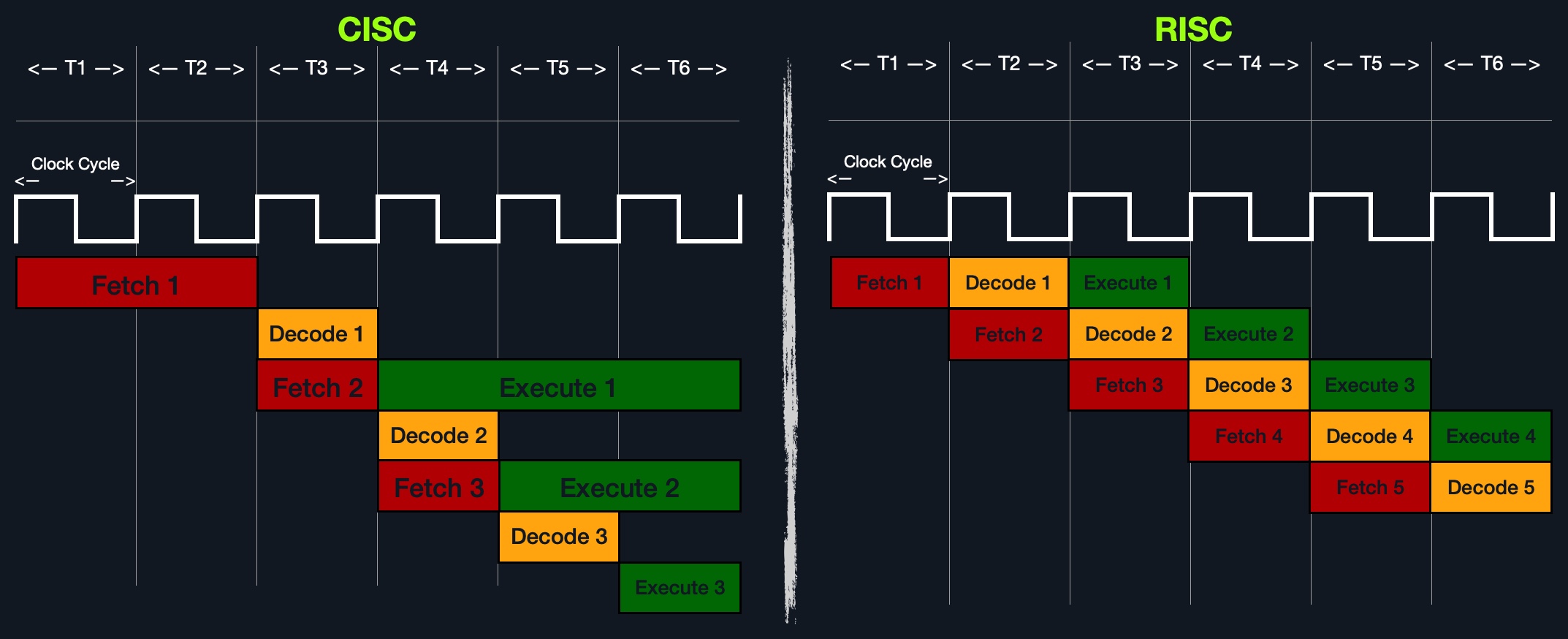

Executing each instruction stage in a single clock cycle and only executing simple instructions leads to RISC processors consuming a fraction of the power consumed by CISC processors, which makes these processors ideal for devices that run on batteries, like smartphones and laptops.

---

CISC vs. RISC

The following table summarizes the main differences between CISC and RISC:

Area	CISC	RISC
Complexity	Favors complex instructions	Favors simple instructions
Length of instructions	Longer instructions - Variable length 'multiples of 8-bits'	Shorter instructions - Fixed length '32-bit/64-bit'
Total instructions per program	Fewer total instructions - Shorter code	More total instructions - Longer code
Optimization	Relies on hardware optimization (in CPU)	Relies on software optimization (in Assembly)
Instruction Execution Time	Variable - Multiple clock cycles	Fixed - One clock cycle
Instructions supported by CPU	Many instructions (~1500)	Fewer instructions (~200)
Power Consumption	High	Very low
Examples	Intel, AMD	ARM, Apple

In the past, having a longer assembly code due to a larger number of total instructions per program was a significant disadvantage for RISC processors due to the limited resources in memory and storage. However, today this is no longer as big of an issue, as memory and storage are not as expensive and limited as they used to be in the past.

Furthermore, with new assemblers and compilers writing extremely optimized code on the software level, RISC processors are becoming faster than CISC processors, even in executing and processing heavy applications, all while consuming much less power.

All of this is making RISC processors more common in recent years. RISC may become the dominant architecture in the upcoming years. But as we speak, the overwhelming majority of computers and servers we will be pentesting are running on Intel/AMD processors with the CISC architecture, making learning CISC assembly our priority. As the basics of all Assembly language variants are pretty similar, learning ARM Assembly should be more straightforward after completing this module.

---

Registers, Addresses, and Data Types

---

Now that we understand general computer and processor architecture, we need to understand a few assembly elements before we start learning Assembly: Registers, Memory Addresses, Address Endianness, and Data Types. Each of these elements is important, and properly understanding them will help us avoid issues and hours of troubleshooting while writing and debugging assembly code.

---

Registers

As previously mentioned, each CPU core has a set of registers. The registers are the fastest components in any computer, as they are built within the CPU core. However, registers are very limited in size and can only hold a few bytes of data at a time. There are many registers in the x86 architecture, but we will only focus on the ones necessary for learning basic Assembly and essential for future binary exploitation.

There are two main types of registers we will be focusing on: Data Registers and Pointer Registers.

Data Registers	Pointer Registers
rax	rbp
rbx	rsp
rcx	rip
rdx
r8
r9
r10

• Data Registers - are usually used for storing instructions/syscall arguments. The primary data registers are: rax, rbx, rcx, and rdx. The rdi and rsi registers also exist and are usually used for the instruction destination and source operands. Then, we have secondary data registers that can be used when all previous registers are in use, which are r8, r9, and r10.
• Pointer Registers - are used to store specific important address pointers. The main pointer registers are the Base Stack Pointer rbp, which points to the beginning of the Stack, the Current Stack Pointer rsp, which points to the current location within the Stack (top of the Stack), and the Instruction Pointer rip, which holds the address of the next instruction.

---

Sub-Registers

Each 64-bit register can be further divided into smaller sub-registers containing the lower bits, at one byte 8-bits, 2 bytes 16-bits, and 4 bytes 32-bits. Each sub-register can be used and accessed on its own, so we don't have to consume the full 64-bits if we have a smaller amount of data.

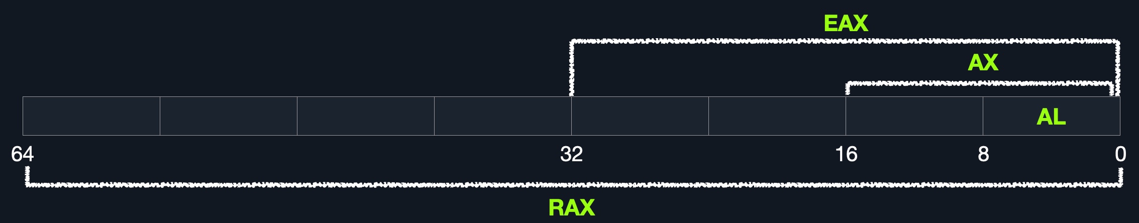
Sub-registers can be accessed as:

Size in bits	Size in bytes	Name	Example
16-bit	2 bytes	the base name	ax
8-bit	1 bytes	base name and/or ends with l	al
32-bit	4 bytes	base name + starts with the e prefix	eax
64-bit	8 bytes	base name + starts with the r prefix	rax

For example, for the bx data register, the 16-bit is bx, so the 8-bit is bl, the 32-bit would be ebx, and the 64-bit would be rbx. The same goes for pointer registers. If we take the base stack pointer bp, its 16-bit sub-register is bp, so the 8-bit is bpl, the 32-bit is ebp, and the 64-bit is rbp.

The following are the names of the sub-registers for all of the essential registers in an x86_64 architecture:

Description	64-bit Register	32-bit Register	16-bit Register	8-bit Register
Data/Arguments Registers
Syscall Number/Return value	rax	eax	ax	al
Callee Saved	rbx	ebx	bx	bl
1st arg - Destination operand	rdi	edi	di	dil
2nd arg - Source operand	rsi	esi	si	sil
3rd arg	rdx	edx	dx	dl
4th arg - Loop counter	rcx	ecx	cx	cl
5th arg	r8	r8d	r8w	r8b
6th arg	r9	r9d	r9w	r9b
Pointer Registers
Base Stack Pointer	rbp	ebp	bp	bpl
Current/Top Stack Pointer	rsp	esp	sp	spl
Instruction Pointer 'call only'	rip	eip	ip	ipl

As we go through the module, we'll discuss how to use each of these registers.

There are other various registers, but we will not cover them in this module, as they are not needed for basic Assembly usage. As an example, there's the RFLAGS register, which is used to maintain various flags used by the CPU, like the zero flag ZF, which is used for conditional instructions.

---

Memory Addresses

As previously mentioned, x86 64-bit processors have 64-bit wide addresses that range from 0x0 to 0xffffffffffffffff, so we expect the addresses to be in this range. However, RAM is segmented into various regions, like the Stack, the heap, and other program and kernel-specific regions. Each memory region has specific read, write, execute permissions that specify whether we can read from it, write to it, or call an address in it.

Whenever an instruction goes through the Instruction Cycle to be executed, the first step is to fetch the instruction from the address it's located at, as previously discussed. There are several types of address fetching (i.e., addressing modes) in the x86 architecture:

Addressing Mode	Description	Example
Immediate	The value is given within the instruction	add 2
Register	The register name that holds the value is given in the instruction	add rax
Direct	The direct full address is given in the instruction	call 0xffffffffaa8a25ff
Indirect	A reference pointer is given in the instruction	call 0x44d000 or call [rax]
Stack	Address is on top of the stack	add rsp

In the above table, lower is slower. The less immediate the value is, the slower it is to fetch it.

Even though speed isn't our biggest concern when learning basic Assembly, we should understand where and how each address is located. Having this understanding will help us in future binary exploitation, with Buffer Overflow exploits, for example. The same understanding will have an even more significant implication with advanced binary exploitation, like ROP or Heap exploitation.

---

Address Endianness

An address endianness is the order of its bytes in which they are stored or retrieved from memory. There are two types of endianness: Little-Endian and Big-Endian. With Little-Endian processors, the little-end byte of the address is filled/retrieved first right-to-left, while with Big-Endian processors, the big-end byte is filled/retrieved first left-to-right.

For example, if we have the address 0x0011223344556677 to be stored in memory, little-endian processors would store the 0x00 byte on the right-most bytes, and then the 0x11 byte would be filled after it, so it becomes 0x1100, and then the 0x22 byte, so it becomes 0x221100, and so on. Once all bytes are in place, they would look like 0x7766554433221100, which is the reverse of the original value. Of course, when retrieving the value back, the processor will also use little-endian retrieval, so the value retrieved would be the same as the original value.

Another example that shows how this can affect the stored values is binary. For example, if we had the 2-byte integer 426, its binary representation is 00000001 10101010. The order in which these two bytes are stored would change its value. For example, if we stored it in reverse as 10101010 00000001, its value becomes 43521.

The big-endian processors would store these bytes as 00000001 10101010 left-to-right, while little-endian processors store them as 10101010 00000001 right-to-left. When retrieving the value, the processor has to use the same endianness used when storing them, or it will get the wrong value. This indicates that the order in which the bytes are stored/retrieved makes a big difference.

The following table demonstrates how endianness works:

Address	0	1	2	3	4	5	6	7	Address Value
Little Endian	77	66	55	44	33	22	11	00	0x
Big Endian	00	11	22	33	44	55	66	77	0x

Address: 0x0011223344556677

Load Address\

You can click on the "Load Address" button to visualize how each endianness loads data/addresses into memory.

As we can see, this means that an address written in little-endian or in big-endian would refer to different locations in the memory, as it would be read differently by each processor type.

This module will always use little-endian byte order, as it is used with Intel/AMD x86 in most modern operating systems, so the shellcode is always represented right-to-left.

The important thing we need to take from this is knowing that our bytes are stored into memory from right-to-left. So, if we were to push an address or a string with Assembly, we would have to push it in reverse. For example, if we want to store the word Hello, we would push its bytes in reverse: o, l, l, e, and finally H.

This may seem a bit counter-intuitive since most people are used to reading from left-to-right. However, this has multiple advantages when processing data, like being able to retrieve a sub-register without having to go through the entire register or being able to perform arithmetic in the correct order right-to-left.

---

Data Types

Finally, the x86 architecture supports many types of data sizes, which can be used with various instructions. The following are the most common data types we will be using with instructions:

Component	Length	Example
byte	8 bits	0xab
word	16 bits - 2 bytes	0xabcd
double word (dword)	32 bits - 4 bytes	0xabcdef12
quad word (qword)	64 bits - 8 bytes	0xabcdef1234567890

Whenever we use a variable with a certain data type or use a data type with an instruction, both operands should be of the same size.

For example, we can't use a variable defined as byte with rax, as rax has a size of 8 bytes. In this case, we would have to use al, which has the same size of 1 byte. The following table shows the appropriate data type for each sub-register:

Sub-register	Data Type
al	byte
ax	word
eax	dword
rax	qword

We will discuss this further in the upcoming sections. With all fundamentals of Assembly covered, we can start learning about x86 assembly instructions and writing basic Assembly code.

---

Assembly File Structure

---

As we learn various Assembly instructions in the coming sections, we'll constantly be writing code, assembling it, and debugging it. This is the best way to learn what each instruction does. So, we need to learn the basic structure of an Assembly code file and then assemble it and debug it.

In this section, we'll go through the basic structure of an Assembly file, and in the following two sections, we will cover assembling it and debugging it. We will be working on a template Hello World! Assembly code as a sample, to first learn the general structure of an assembly file and then how to assemble it and debug it. Let us start by taking a look at and dissecting a sample Hello World! Assembly code template:

Code: nasm

         global  _start

         section .data
message: db      "Hello HTB Academy!"

         section .text
_start:
         mov     rax, 1
         mov     rdi, 1
         mov     rsi, message
         mov     rdx, 18
         syscall

         mov     rax, 60
         mov     rdi, 0
         syscall

This Assembly code (once assembled and linked) should print the string 'Hello HTB Academy!' to the screen. We won't go into detail on how this is processed just yet, but we need to understand the main elements of the code template.

---

Assembly File Structure

First, let's examine the way the code is distributed:

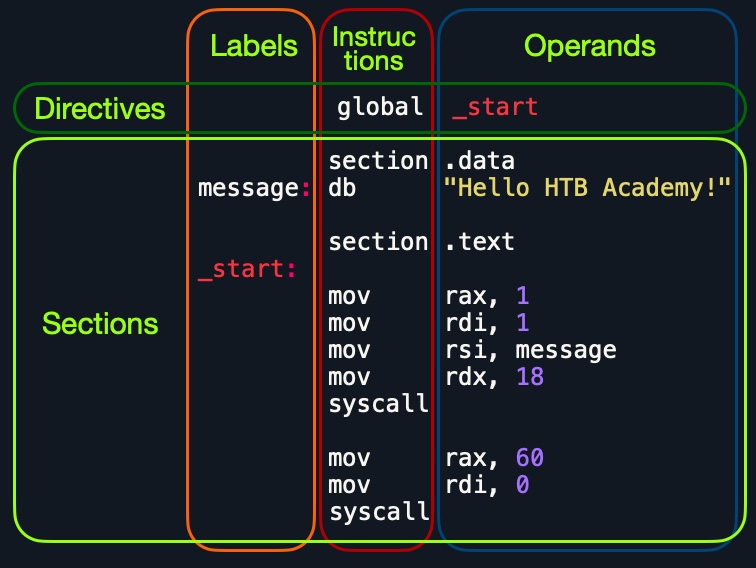
Looking at the vertical parts of the code, each line can have three elements:

1. Labels	2. Instructions	3. Operands

We have discussed the instructions and their operands in the previous sections, and we'll go into detail on various assembly instructions in the coming sections. In addition to that, we can define a label at each line. Each label can be referred to by instructions or by directives.

Next, if we look at the code line-by-line, we see that it has three main parts:

Section	Description
global _start	This is a directive that directs the code to start executing at the _start label defined below.
section .data	This is the data section, which should contain all of the variables.
section .text	This is the text section containing all of the code to be executed.

Both the .data and .text sections refer to the data and text memory segments, in which these instructions will be stored.

---

Directives

An Assembly code is line-based, which means that the file is processed line-by-line, executing the instruction of each line. We see at the first line a directive global _start, which instructs the machine to start processing the instructions after the _start label. So, the machine goes to the _start label and starts executing the instructions there, which will print the message on the screen. This will be covered more thoroughly in the Control Instructions sections.

---

Variables

Next, we have the .data section. The data section holds our variables to make it easier for us to define variables and reuse them without writing them multiple times. Once we run our program, all of our variables will be loaded into memory in the data segment.

When we run the program, it will load any variables we have defined into memory so that they will be ready for usage when we call them. We will notice later in the module that by the time we start executing instructions at the _start label, all of our variables will be already loaded into memory.

We can define variables using db for a list of bytes, dw for a list of words, dd for a list of digits, and so on. We can also label any of our variables so we can call it or reference it later. The following are some examples of defining variables:

Instruction	Description
db 0x0a	Defines the byte 0x0a, which is a new line.
message db 0x41, 0x42, 0x43, 0x0a	Defines the label message => abc.
message db "Hello World!", 0x0a	Defines the label message => Hello World!.

Furthermore, we can use the equ instruction with the $ token to evaluate an expression, like the length of a defined variable's string. However, the labels defined with the equ instruction are constants, and they cannot be changed later.

For example, the following code defines a variable and then defines a constant for its length:

Code: nasm

section .data
    message db "Hello World!", 0x0a
    length  equ $-message

Note: the $ token indicates the current distance from the beginning of the current section. As the message variable is at the beginning of the data section, the current location, i.e,. value of $, equals the length of the string. For the scope of this module, we will only use this token to calculate lengths of strings, using the same line of code shown above.

---

Code

The second (and most important) section is the .text section. This section holds all of the assembly instructions and loads them to the text memory segment. Once all instructions are loaded into the text segment, the processor starts executing them one after another.

The default convention is to have the _start label at the beginning of the .text section, which -as per the global _start directive- starts the main code that will be executed as the program runs. As we will see later in the module, we can define other labels within the .text section, for loops and other functions.

The text segment within the memory is read-only, so we cannot write any variables within it. The data section, on the other hand, is read/write, which is why we write our variables to it. However, the data segment within the memory is not executable, so any code we write to it cannot be executed. This separation is part of memory protections to mitigate things like buffer overflows and other types of binary exploitation.

Tip: We can add comments to our assembly code with a semi-colon ;. We can use comments to explain the purpose of each part of the code, and what each line is doing. Doing so will save us a lot of time in the future if we ever revisit the code and need to understand it.

With this, we should understand the basic structure of an Assembly file.

---

Assembling & Disassembling

---

Now that we understand the basic structure and elements of an Assembly file, we can start assembling it using the nasm tool. The entire assembly file structure we learned in the previous section is based on the nasm file structure. Upon assembling our code with nasm, it understands the various parts of the file and then correctly assembles them to be properly run during run time.

After we assemble our code with nasm, we can link it using ld to utilize various OS features and libraries.

---

Assembling

First, we will copy the code below into a file called helloWorld.s.

Note: assembly files usually use the .s or the .asm extensions. We will be using .s in this module.

We don't have to keep using tabs to separate parts of an assembly file, as this was only for demonstration purposes. We can write the following code into our helloWorld.s file:

Code: nasm

global _start

section .data
    message db "Hello HTB Academy!"
    length equ $-message

section .text
_start:
    mov rax, 1
    mov rdi, 1
    mov rsi, message
    mov rdx, length
    syscall

    mov rax, 60
    mov rdi, 0
    syscall

Note how we used equ to dynamically calculate the length of message, instead of using a static 18. This will become very handy later on. Once we do, we will assemble the file using nasm, with the following command:

Assembling & Disassembling

root@htb[/htb]$ nasm -f elf64 helloWorld.s

Note: The -f elf64 flag is used to note that we want to assemble a 64-bit assembly code. If we wanted to assemble a 32-bit code, we would use -f elf.

This should output a helloWorld.o object file, which is then assembled into machine code, along with the details of all variables and sections. This file is not executable just yet.

---

Linking

The final step is to link our file using ld. The helloWorld.o object file, though assembled, still cannot be executed. This is because many references and labels used by nasm need to be resolved into actual addresses, along with linking the file with various OS libraries that may be needed.

This is why a Linux binary is called ELF, which stands for an Executable and Linkable Format. To link a file using ld, we can use the following command:

Assembling & Disassembling

root@htb[/htb]$ ld -o helloWorld helloWorld.o

Note: if we were to assemble a 32-bit binary, we need to add the '-m elf_i386' flag.

Once we link the file with ld, we should have the final executable file:

Assembling & Disassembling

root@htb[/htb]$ ./helloWorld
Hello HTB Academy!

We have successfully assembled and linked our first assembly file. We will be assembling, linking, and running our code frequently through this module, so let us build a simple bash script to make it easier:

Code: bash

#!/bin/bash

fileName="${1%%.*}" # remove .s extension

nasm -f elf64 ${fileName}".s"
ld ${fileName}".o" -o ${fileName}
[ "$2" == "-g" ] && gdb -q ${fileName} || ./${fileName}

Now we can write this script to assembler.sh, chmod +x it, and then run it on our assembly file. It will assemble it, link it, and run it:

Assembling & Disassembling

root@htb[/htb]$ ./assembler.sh helloWorld.s
Hello HTB Academy!

Great! Before we move on, let's disassemble and examine our files to learn more about the process we just did.

---

Disassembling

To disassemble a file, we will use the objdump tool, which dumps machine code from a file and interprets the assembly instruction of each hex code. We can disassemble a binary using the -D flag.

Note: we will also use the flag -M intel, so that objdump would write the instructions in the Intel syntax, which we are using, as we discussed before.

Let's start by disassembling our final ELF executable file:

Assembling & Disassembling

root@htb[/htb]$ objdump -M intel -d helloWorld

helloWorld:     file format elf64-x86-64

Disassembly of section .text:

0000000000401000 <_start>:
  401000:    b8 01 00 00 00           mov    eax,0x1
  401005:    bf 01 00 00 00           mov    edi,0x1
  40100a:    48 be 00 20 40 00 00     movabs rsi,0x402000
  401011:    00 00 00
  401014:    ba 12 00 00 00           mov    edx,0x12
  401019:    0f 05                    syscall
  40101b:    b8 3c 00 00 00           mov    eax,0x3c
  401020:    bf 00 00 00 00           mov    edi,0x0
  401025:    0f 05                    syscall

We see that our original assembly code is highly preserved, with the only change being 0x402000 used in place of the message variable and replacing the length constant with its value of 0x12. We also see that nasm efficiently changed our 64-bit registers to the 32-bit sub-registers where possible, to use less memory when possible, like changing mov rax, 1 to mov eax,0x1.

If we wanted to only show the assembly code, without machine code or addresses, we could add the --no-show-raw-insn --no-addresses flags, as follows:

Assembling & Disassembling

root@htb[/htb]$ objdump -M intel --no-show-raw-insn --no-addresses -d helloWorld

helloWorld:     file format elf64-x86-64

Disassembly of section .text:

<_start>:
        mov    eax,0x1
        mov    edi,0x1
        movabs rsi,0x402000
        mov    edx,0x12
        syscall 
        mov    eax,0x3c
        mov    edi,0x0
        syscall

Note: Note that objdump has changed the third instruction into movabs. This is the same as mov, so in case you need to reassemble the code, you can change it back to mov.

The -d flag will only disassemble the .text section of our code. To dump any strings, we can use the -s flag, and add -j .data to only examine the .data section. This means that we also do not need to add -M intel. The final command is as follows:

Assembling & Disassembling

root@htb[/htb]$ objdump -sj .data helloWorld

helloWorld:     file format elf64-x86-64

Contents of section .data:
 402000 48656c6c 6f204854 42204163 6164656d  Hello HTB Academ
 402010 7921                                 y!

As we can see, the .data section indeed contains the message variable with the string Hello HTB Academy!. This should give us a better idea of how our code was assembled into machine code and how it looks after we assemble it. Next, let us go through the basics of code debugging, which is a critical skill we need to learn.

---

GNU Debugger (GDB)

---

Debugging is an important skill to learn for developers and pentesters alike. Debugging is a term used for finding and removing issues (i.e., bugs) from our code, hence the name de-bugging. When we develop a program, we will very frequently run into bugs in our code. It is not efficient to keep changing our code until it does what we expect of it. Instead, we perform debugging by setting breakpoints and seeing how our program acts on each of them and how our input changes between them, which should give us a clear idea of what is causing the bug.

Programs written in high-level languages can set breakpoints on specific lines and run the program through a debugger to monitor how they act. With Assembly, we deal with machine code represented as assembly instructions, so our breakpoints are set in the memory location in which our machine code is loaded, as we will see.

To debug our binaries, we will be using a well-known debugger for Linux programs called GNU Debugger (GDB). There are other similar debuggers for Linux, like Radare and Hopper, and for Windows, like Immunity Debugger and WinGDB. There are also powerful debuggers available for many platforms, like IDA Pro and EDB. In this module, we will be using GDB. It is the most reliable for Linux binaries since it is built and maintained directly by GNU, which gives it an excellent integration with the Linux system and its components.

---

Installation

GDB is installed in many Linux distributions, and it is also installed by default in Parrot OS and PwnBox. In case it is not installed in your VM, you can use apt to install it with the following commands:

GNU Debugger (GDB)

root@htb[/htb]$ sudo apt-get update
root@htb[/htb]$ sudo apt-get install gdb

One of the great features of GDB is its support for third-party plugins. An excellent plugin that is well maintained and has good documentation is GEF. GEF is a free and open-source GDB plugin that is built precisely for reverse engineering and binary exploitation. This fact makes it a great tool to learn.

To add GEF to GDB, we can use the following commands:

GNU Debugger (GDB)

root@htb[/htb]$ wget -O ~/.gdbinit-gef.py -q https://gef.blah.cat/py
root@htb[/htb]$ echo source ~/.gdbinit-gef.py >> ~/.gdbinit

---

Getting Started

Now that we have both tools installed, we can run gdb to debug our HelloWorld binary using the following commands, and GEF will be loaded automatically:

GNU Debugger (GDB)

root@htb[/htb]$ gdb -q ./helloWorld
...SNIP...
gef➤

As we can see from gef➤, GEF is loaded when GDB is run. If you ever run into any issues with GEF, you can consult with the GEF Documentation, and you will likely find a solution.

Going forward, we will frequently be assembling and linking our assembly code and then running it with gdb. To do so quickly, we can use the assembler.sh script we wrote in the previous section with the -g flag. It will assemble and link the code, and then run it with gdb, as follows:

GNU Debugger (GDB)

root@htb[/htb]$ ./assembler.sh helloWorld.s -g
...SNIP...
gef➤

---

Info

Once GDB is started, we can use the info command to view general information about the program, like its functions or variables.

Tip: If we want to understand how any command runs within GDB, we can use the help CMD command to get its documentation. For example, we can try executing help info

Functions

To start, we will use the info command to check which functions are defined within the binary:

GNU Debugger (GDB)

gef➤  info functions

All defined functions:

Non-debugging symbols:
0x0000000000401000  _start

As we can see, we found our main _start function.

Variables

We can also use the info variables command to view all available variables within the program:

GNU Debugger (GDB)

gef➤  info variables

All defined variables:

Non-debugging symbols:
0x0000000000402000  message
0x0000000000402012  __bss_start
0x0000000000402012  _edata
0x0000000000402018  _end

As we can see, we find the message, along with some other default variables that define memory segments. We can do many things with functions, but we will focus on two main points: Disassembly and Breakpoints.

---

Disassemble

To view the instructions within a specific function, we can use the disassemble or disas command along with the function name, as follows:

GNU Debugger (GDB)

gef➤  disas _start

Dump of assembler code for function _start:
   0x0000000000401000 <+0>:    mov    eax,0x1
   0x0000000000401005 <+5>:    mov    edi,0x1
   0x000000000040100a <+10>:    movabs rsi,0x402000
   0x0000000000401014 <+20>:    mov    edx,0x12
   0x0000000000401019 <+25>:    syscall
   0x000000000040101b <+27>:    mov    eax,0x3c
   0x0000000000401020 <+32>:    mov    edi,0x0
   0x0000000000401025 <+37>:    syscall
End of assembler dump.

As we can see, the output we got closely resembles our assembly code and the disassembly output we got from objdump in the previous section. We need to focus on the main thing from this disassembly: the memory addresses for each instruction and operands (i.e., arguments).

Having the memory address is critical for examining the variables/operands and setting breakpoints for a certain instruction.

You may notice through debugging that some memory addresses are in the form of 0x00000000004xxxxx, rather than their raw address in memory 0xffffffffaa8a25ff. This is due to $rip-relative addressing in Position-Independent Executables PIE, in which the memory addresses are used relative to their distance from the instruction pointer $rip within the program's own Virtual RAM, rather than using raw memory addresses. This feature may be disabled to reduce the risk of binary exploitation.

Next, let us go through the basics of debugging with GDB by using breakpoints, examining data, and stepping through the program.

---

Debugging with GDB

---

Now that we have the general information about our program, we will start running it and debugging it. Debugging consists mainly of four steps:

Step	Description
Break	Setting breakpoints at various points of interest
Examine	Running the program and examining the state of the program at these points
Step	Moving through the program to examine how it acts with each instruction and with user input
Modify	Modify values in specific registers or addresses at specific breakpoints, to study how it would affect the execution

We will go through these points in this section to learn the basics of debugging a program with GDB.

---

Break

The first step of debugging is setting breakpoints to stop the execution at a specific location or when a particular condition is met. This helps us in examining the state of the program and the value of registers at that point. Breakpoints also allow us to stop the program's execution at that point so that we can step into each instruction and examine how it changes the program and values.

We can set a breakpoint at a specific address or for a particular function. To set a breakpoint, we can use the break or b command along with the address or function name we want to break at. For example, to follow all instructions run by our program, let's break at the _start function, as follows:

Debugging with GDB

gef➤  b _start

Breakpoint 1 at 0x401000

Now, in order to start our program, we can use the run or r command:

gef➤  b _start
Breakpoint 1 at 0x401000
gef➤  r
Starting program: ./helloWorld 

Breakpoint 1, 0x0000000000401000 in _start ()
[ Legend: Modified register | Code | Heap | Stack | String ]
───────────────────────────────────────────────────────────────────────────────────── registers ────
$rax   : 0x0               
$rbx   : 0x0               
$rcx   : 0x0               
$rdx   : 0x0               
$rsp   : 0x00007fffffffe310  →  0x0000000000000001
$rbp   : 0x0               
$rsi   : 0x0               
$rdi   : 0x0               
$rip   : 0x0000000000401000  →  <_start+0> mov eax, 0x1
...SNIP...
───────────────────────────────────────────────────────────────────────────────────────── stack ────
0x00007fffffffe310│+0x0000: 0x0000000000000001     ← $rsp
0x00007fffffffe318│+0x0008: 0x00007fffffffe5a0  →  "./helloWorld"
...SNIP...
─────────────────────────────────────────────────────────────────────────────────── code:x86:64 ────
     0x400ffa                  add    BYTE PTR [rax], al
     0x400ffc                  add    BYTE PTR [rax], al
     0x400ffe                  add    BYTE PTR [rax], al
 →   0x401000 <_start+0>       mov    eax, 0x1
     0x401005 <_start+5>       mov    edi, 0x1
     0x40100a <_start+10>      movabs rsi, 0x402000
     0x401014 <_start+20>      mov    edx, 0x12
     0x401019 <_start+25>      syscall 
     0x40101b <_start+27>      mov    eax, 0x3c
─────────────────────────────────────────────────────────────────────────────────────── threads ────
[#0] Id 1, Name: "helloWorld", stopped 0x401000 in _start (), reason: BREAKPOINT
───────────────────────────────────────────────────────────────────────────────────────── trace ────
[#0] 0x401000 → _start()
────────────────────────────────────────────────────────────────────────────────────────────────────

If we want to set a breakpoint at a certain address, like _start+10, we can either b *_start+10 or b *0x40100a:

Debugging with GDB

gef➤  b *0x40100a
Breakpoint 1 at 0x40100a

The * tells GDB to break at the instruction stored in 0x40100a.

Note: Once the program is running, if we set another breakpoint, like b *0x401005, in order to continue to that breakpoint, we should use the continue or c command. If we use run or r again, it will run the program from the start. This can be useful to skip loops, as we will see later in the module.

If we want to see what breakpoints we have at any point of the execution, we can use the info breakpoint command. We can also disable, enable, or delete any breakpoint. Furthermore, GDB also supports setting conditional breaks that stop the execution when a specific condition is met.

---

Examine

The next step of debugging is examining the values in registers and addresses. As we can see in the previous terminal output, GEF automatically gave us a lot of helpful information when we hit our breakpoint. This is one of the benefits of having the GEF plugin, as it automates many steps that we usually take at every breakpoint, like examining the registers, the stack, and the current assembly instructions.

To manually examine any of the addresses or registers or examine any other, we can use the x command in the format of x/FMT ADDRESS, as help x would tell us. The ADDRESS is the address or register we want to examine, while FMT is the examine format. The examine format FMT can have three parts:

Argument	Description	Example
Count	The number of times we want to repeat the examine	2, 3, 10
Format	The format we want the result to be represented in	x(hex), s(string), i(instruction)
Size	The size of memory we want to examine	b(byte), h(halfword), w(word), g(giant, 8 bytes)

Instructions

For example, if we wanted to examine the next four instructions in line, we will have to examine the $rip register (which holds the address of the next instruction), and use 4 for the count, i for the format, and g for the size (for 8-bytes or 64-bits). So, the final examine command would be x/4ig $rip, as follows:

Debugging with GDB

gef➤  x/4ig $rip

=> 0x401000 <_start>:    mov    eax,0x1
   0x401005 <_start+5>:    mov    edi,0x1
   0x40100a <_start+10>:    movabs rsi,0x402000
   0x401014 <_start+20>:    mov    edx,0x12

We see that we get the following four instructions as expected. This can help us as we go through a program in examining certain areas and what instructions they may contain.

Strings

We can also examine a variable stored at a specific memory address. We know that our message variable is stored at the .data section on address 0x402000 from our previous disassembly. We also see the upcoming command movabs rsi, 0x402000, so we may want to examine what is being moved from 0x402000.

In this case, we will not put anything for the Count, as we only want one address (1 is the default), and will use s as the format to get it in a string format rather than in hex:

Debugging with GDB

gef➤  x/s 0x402000

0x402000:    "Hello HTB Academy!"

As we can see, we can see the string at this address represented as text rather than hex characters.

Note: if we don't specify the Size or Format, it will default to the last one we used.

Addresses

The most common format of examining is hex x. We often need to examine addresses and registers containing hex data, such as memory addresses, instructions, or binary data. Let us examine the same previous instruction, but in hex format, to see how it looks:

Debugging with GDB

gef➤  x/wx 0x401000

0x401000 <_start>:    0x000001b8

We see instead of mov eax,0x1, we get 0x000001b8, which is the hex representation of the mov eax,0x1 machine code in little-endian formatting.

• This is read as: b8 01 00 00.

Try repeating the commands we used for examining strings using x to examine them in hex. We should see the same text but in hex format. We can also use GEF features to examine certain addresses. For example, at any point we can use the registers command to print out the current value of all registers:

gdb

gef➤  registers
$rax   : 0x0               
$rbx   : 0x0               
$rcx   : 0x0               
$rdx   : 0x0               
$rsp   : 0x00007fffffffe310  →  0x0000000000000001
$rbp   : 0x0               
$rsi   : 0x0               
$rdi   : 0x0               
$rip   : 0x0000000000401000  →  <_start+0> mov eax, 0x1
...SNIP...

---

Step

The third step of debugging is stepping through the program one instruction or line of code at a time. As we can see, we are currently at the very first instruction in our helloWorld program:

gdb

─────────────────────────────────────────────────────────────────────────────────── code:x86:64 ────
     0x400ffe                  add    BYTE PTR [rax], al
 →   0x401000 <_start+0>       mov    eax, 0x1
     0x401005 <_start+5>       mov    edi, 0x1

Note: the instruction shown with the -> symbol is where we are at, and it has not yet been processed.

To move through the program, there are three different commands we can use: stepi and step.

Step Instruction

The stepi or si command will step through the assembly instructions one by one, which is the smallest level of steps possible while debugging. Let us use the si command to see how we get to the next instruction:

gdb

─────────────────────────────────────────────────────────────────────────────────── code:x86:64 ────
gef➤  si
0x0000000000401005 in _start ()
   0x400fff                  add    BYTE PTR [rax+0x1], bh
 →   0x401005 <_start+5>       mov    edi, 0x1
     0x40100a <_start+10>      movabs rsi, 0x402000
     0x401014 <_start+20>      mov    edx, 0x12
     0x401019 <_start+25>      syscall 
─────────────────────────────────────────────────────────────────────────────────────── threads ────
     [#0] Id 1, Name: "helloWorld", stopped 0x401005 in _start (), reason: SINGLE STEP

As we can see, we took exactly one step and stopped again at the mov edi, 0x1 instruction.

Step Count

Similarly to examine, we can repeat the si command by adding a number after it. For example, if we wanted to move 3 steps to reach the syscall instruction, we can do so as follows:

gdb

gef➤  si 3
0x0000000000401019 in _start ()
─────────────────────────────────────────────────────────────────────────────────── code:x86:64 ────
     0x401004 <_start+4>       add    BYTE PTR [rdi+0x1], bh
     0x40100a <_start+10>      movabs rsi, 0x402000
     0x401014 <_start+20>      mov    edx, 0x12
 →   0x401019 <_start+25>      syscall 
     0x40101b <_start+27>      mov    eax, 0x3c
     0x401020 <_start+32>      mov    edi, 0x0
     0x401025 <_start+37>      syscall 
─────────────────────────────────────────────────────────────────────────────────────── threads ────
[#0] Id 1, Name: "helloWorld", stopped 0x401019 in _start (), reason: SINGLE STEP

As we can see, we stopped at the syscall instruction as expected.

Tip: You can hit the return/enter empty in order to repeat the last command. Try hitting it at this stage, and you should make another 3 steps, and break at the other syscall instruction.

Step

The step or s command, on the other hand, will continue until the following line of code is reached or until it exits from the current function. If we run an assembly code, it will break when we exit the current function _start.

If there's a call to another function within this function, it'll break at the beginning of that function. Otherwise, it'll break after we exit this function after the program's end. Let us try using s, and see what happens:

Debugging with GDB

gef➤  step

Single stepping until exit from function _start,
which has no line number information.
Hello HTB Academy!
[Inferior 1 (process 14732) exited normally]

We see that the execution continued until we reached the exit from the _start function, so we reached the end of the program and exited normally without any errors. We also see that GDB printed the program's output Hello HTB Academy! as well.

Note: There's also the next or n command, which will also continue until the next line, but will skip any functions called in the same line of code, instead of breaking at them like step. There's also the nexti or ni, which is similar to si, but skips functions calls, as we will see later on in the module.

---

Modify

The final step of debugging is modifying values in registers and addresses at a certain point of execution. This helps us in seeing how this would affect the execution of the program.

Addresses

To modify values in GDB, we can use the set command. However, we will utilize the patch command in GEF to make this step much easier. Let's enter help patch in GDB to get its help menu:

Debugging with GDB

gef➤  help patch

Write specified values to the specified address.
Syntax: patch (qword|dword|word|byte) LOCATION VALUES
patch string LOCATION "double-escaped string"
...SNIP...

As we can see, we have to provide the type/size of the new value, the location to be stored, and the value we want to use. So, let's try changing the string stored in the .data section (at address 0x402000 as we saw earlier) to the string Patched!.

We will break at the first syscall at 0x401019, and then do the patch, as follows:

Debugging with GDB

gef➤  break *0x401019

Breakpoint 1 at 0x401019
gef➤  r
gef➤  patch string 0x402000 "Patched!\\x0a"
gef➤  c

Continuing.
Patched!
 Academy!

We see that we successfully modified the string and got Patched!\n Academy! instead of the old string. Notice how we used \x0a for adding a new line after our string.

Registers

We also note that we did not replace the entire string. This is because we only modified the characters up to the length of our string and left the remainder of the old string. Finally, the write system call specified a length of 0x12 of bytes to be printed.

To fix this, let's modify the value stored in $rdx to the length of our string, which is 0x9. We will only patch a size of one byte. We will go into details of how syscall works later in the module. Let us demonstrate using set to modify $rdx, as follows:

Debugging with GDB

gef➤  break *0x401019

Breakpoint 1 at 0x401019
gef➤  r
gef➤  patch string 0x402000 "Patched!\\x0a"
gef➤  set $rdx=0x9
gef➤  c

Continuing.
Patched!

We see that we successfully modified the final printed string and have the program output something of our choosing. The ability to modify values of registers and addresses will help us a lot through debugging and binary exploitation, as it allows us to test various values and conditions without having to change the code and recompile the binary every time.

---

Conclusion

The ability to set breakpoints to stop the execution, step through a program and each of its instructions, examine various data and addresses at each point, and modify values when needed, enables us to do proper debugging and reverse engineering.

Whether we want to see exactly why our program is failing or understand how a program is running and what it's doing at each point, GDB becomes very handy.

For penetration testing, this process enables us to understand how a program handles input at a certain point and exactly why it's failing. This allows us to develop exploits that take advantage of such failures, as we will learn in the Binary Exploitation modules.

---

Module Project

---

So far, we have learned the basics of computer and CPU architecture and the basics of Assembly language and debugging. We will now start learning various x86 assembly instructions. We are likely to run into these types of instructions during penetration testing and reverse engineering exercises, so understanding how they work gives us the ability to interpret what they are doing and understand what the program is doing.

We will start by learning how to move data and values between registers and memory addresses. Then, we will learn instructions that take one operand (Unary Operations) and instructions with two operands ( Binary Instructions). Later on, we will go through assembly control instructions and shellcoding.

---

Fibonacci Sequence

Before we start, however, let's discuss the program we will be developing throughout this module, using the various instructions we will learn.\ We will be developing a basic Fibonacci sequence calculator using x86 assembly language.

At the simplest term, a Fibonacci number is the sum of the two numbers preceding it in the sequence (i.e. Fn``= Fn-1``+ Fn-2). For example, if we start with F0=0 and F1=1, then F₂ is F1``+ F0, which is F2``= 1 + 0 -> 1.\ Following the same formula, F₃ is F3=1+1=2, F₄ is F4``= 2 + 1 -> 3, and so on.

If we continue until F₁₀, this is the sequence we would have: 0, 1, 1, 2, 3, 5, 8, 13, 21, 34, 55. As we can see, each number equals the sum of the two before it.

---

Golden Ratio

Fibonacci sequence is handy in many fields, like art, mathematics, physics, computer science, and even economics and finance. For example, the Fibonacci sequence is an excellent representation of the golden ratio (or phi Φ), which was used by many artists and architects throughout history and seen everywhere around us in nature:

Furthermore, many modern designers are using the golden ratio in their designs, most famously in the logos of some known brands:

If you are interested in learning more about the Golden Ratio, you can watch this video.

---

Final Program

We will be developing a Fibonacci sequence calculator for this module, which allows us to practice various assembly instructions as we learn them and build the program as we go until we have the complete calculator program by the end.

The program will first ask you for the maximum Fibonacci you want to calculate and then print all Fibonacci numbers up to this number. The following example shows us how it would look:

Module Project

root@htb[/htb]$ ./fib 

Please input max Fn
100
1
1
2
3
5
8
13
21
34
55
89

By the end of the module, you will have developed the above program using nothing but Assembly instructions. We can download the final program from this link and run it to see the final project result.

---

1. \ Page 11
2. Data Movement

Data Movement

---

Let's start with data movement instructions, which are among the most fundamental instructions in any assembly program. We will frequently use data movement instructions for moving data between addresses, moving data between registers and memory addresses, and loading immediate data into registers or memory addresses. The main Data Movement instructions are:

Instruction	Description	Example
mov	Move data or load immediate data	mov rax, 1 -> rax = 1
lea	Load an address pointing to the value	lea rax, [rsp+5] -> rax = rsp+5
xchg	Swap data between two registers or addresses	xchg rax, rbx -> rax = rbx, rbx = rax

---

Moving Data

Let's use the mov instruction as the very first instructions in our module project fibonacci. We will need to load the initial values (F0=0 and F1=1) to rax and rbx, such that rax = 0 and rbx = 1. Let us copy the following code to a fib.s file:

Code: nasm

global  _start

section .text
_start:
    mov rax, 0
    mov rbx, 1

Now, let's assemble this code and run it with gdb to see how the mov instruction works in action:

$ ./assembler.sh fib.s -g
gef➤  b _start
Breakpoint 1 at 0x401000
gef➤  r
─────────────────────────────────────────────────────────────────────────────────── code:x86:64 ────
 →   0x401000 <_start+0>       mov    eax, 0x0
     0x401005 <_start+5>       mov    ebx, 0x1
───────────────────────────────────────────────────────────────────────────────────── registers ────
$rax   : 0x0
$rbx   : 0x0

...SNIP...

─────────────────────────────────────────────────────────────────────────────────── code:x86:64 ────
     0x401000 <_start+0>       mov    eax, 0x0
 →   0x401005 <_start+5>       mov    ebx, 0x1
───────────────────────────────────────────────────────────────────────────────────── registers ────
$rax   : 0x0
$rbx   : 0x1

Like this, we have loaded the initial values into our registers to later perform other operations and instructions on them.

Note: In assembly, moving data does not affect the source operand. So, we can consider mov as a copy function, rather than an actual move.

---

Loading Data

We can load immediate data using the mov instruction. For example, we can load the value of 1 into the rax register using the mov rax, 1 instruction. We have to remember here that the size of the loaded data depends on the size of the destination register. For example, in the above mov rax, 1 instruction, since we used the 64-bit register rax, it will be moving a 64-bit representation of the number 1 (i.e. 0x00000001), which is not very efficient.

This is why it is more efficient to use a register size that matches our data size. For example, we will get the same result as the above example if we use mov al, 1, since we are moving 1-byte (0x01) into a 1-byte register (al), which is much more efficient. This is evident when we look at the disassembly of both instructions in objdump.

Let us take the following basic assembly code to compare the disassembly of both instructions:

Code: nasm

global  _start

section .text
_start:
    mov rax, 0
    mov rbx, 1
    mov bl, 1

Now let's assemble it and view its shellcode with objdump:

Data Movement

root@htb[/htb]$ nasm -f elf64 fib.s && objdump -M intel -d fib.o
...SNIP...
0000000000000000 <_start>:
   0:    b8 00 00 00 00           mov    eax,0x0
   5:    bb 01 00 00 00           mov    ebx,0x1
   a:    b3 01                    mov    bl,0x1

We can see that the shellcode of the first instruction is more than double the size of the last instruction.

This understanding will become very handy when writing shellcodes.

Let us modify our code to use sub-registers to make it more efficient:

Code: nasm

global  _start

section .text
_start:
    mov al, 0
    mov bl, 1

The xchg instruction will swap the data between the two registers. Try adding xchg rax, rbx to the end of the code, assemble it, and then run it through gdb to see how it works.

---

Address Pointers

Another critical concept to understand is using pointers. In many cases, we would see that the register or address we are using does not immediately contain the final value but contains another address that points to the final value. This is always the case with pointer registers, like rsp, rbp, and rip, but is also used with any other register or memory address.

For example, let's assemble and run gdb on our assembled fib binary, and check the rsp and rip registers:

gdb

gdb -q ./fib
gef➤  b _start
Breakpoint 1 at 0x401000
gef➤  r
...SNIP...
$rsp   : 0x00007fffffffe490  →  0x0000000000000001
$rip   : 0x0000000000401000  →  <_start+0> mov eax, 0x0

We see that both registers contain pointer addresses to other locations. GEF does an excellent job of showing us the final destination value.

Moving Pointer Values

We can see that the rsp register holds the final value of 0x1, and its immediate value is a pointer address to 0x1. So, if we were to use mov rax, rsp, we won't be moving the value 0x1 to rax, but we will be moving the pointer address 0x00007fffffffe490 to rax.

To move the actual value, we will have to use square brackets [], which in x86_64 assembly and Intel syntax means load value at address. So, in the same above example, if we wanted to move the final value rsp is pointing to, we can wrap rsp in square brackets, like mov rax, [rsp], and this mov instruction will move the final value rather than the immediate value (which is an address to the final value).

We can use square brackets to compute an address offset relative to a register or another address. For example, we can do mov rax, [rsp+10] to move the value stored 10 address away from rsp.

To properly demonstrate this, let us take the following example code:

Code: nasm

global  _start

section .text
_start:
    mov rax, rsp
    mov rax, [rsp]

This is just a simple program to demonstrate this point and see the difference between the two instructions.

Now, let's assemble the code and run the program with gdb:

gdb

$ ./assembler.sh rsp.s -g
gef➤  b _start
Breakpoint 1 at 0x401000
gef➤  r
...SNIP...
─────────────────────────────────────────────────────────────────────────────────── code:x86:64 ────
 →   0x401000 <_start+0>       mov    rax, rsp
───────────────────────────────────────────────────────────────────────────────────── registers ────
$rax   : 0x00007fffffffe490  →  0x0000000000000001
$rsp   : 0x00007fffffffe490  →  0x0000000000000001

As we can see, the mov rax, rsp moved the immediate value stored at rsp (which is a pointer address to rsp) to the rax register.Now let's press si and check how rax will look after the second instruction:

gdb

$ ./assembler.sh rsp.s -g
gef➤  b _start
Breakpoint 1 at 0x401000
gef➤  r
...SNIP...
─────────────────────────────────────────────────────────────────────────────────── code:x86:64 ────
 →   0x401003 <_start+3>       mov    rax, QWORD PTR [rsp]
───────────────────────────────────────────────────────────────────────────────────── registers ────
$rax   : 0x1               
$rsp   : 0x00007fffffffe490  →  0x0000000000000001

We can see that this time, the final value of 0x1 was moved into the rax register.

Note: When using [], we may need to set the data size before the square brackets, like byte or qword. However, in most cases, nasm will automatically do that for us. We can see above that the final instruction is actually mov rax, QWORD PTR [rsp]. We also see that nasm also added PTR to specify moving a value from a pointer.

Loading Value Pointers

Finally, we need to understand how to load a pointer address to a value, using the lea (or Load Effective Address) instruction, which loads a pointer to the specified value, as in lea rax, [rsp]. This is the opposite of what we just learned above (i.e., load pointer to a value vs. move value from pointer).

In some instances, we need to load the address of a value to a certain register rather than directly load the value in that register. This is usually done when the data is large and would not fit in one register, so the data is placed on the stack or in the heap, and a pointer to its location is stored in the register.

For example, the write syscall we used in our HelloWorld program requires a pointer to the text to be printed, instead of directly providing the text, which may not fit in its entirety in the register, as the register is only 64-bits or 8 bytes.

First, if we wanted to load a direct pointer to a variable or a label, we can still use mov instructions. Since the variable name is a pointer to where it is located in memory, mov will store this pointer to the destination address. For example, both mov rax, rsp and lea rax, [rsp] will do the same thing of storing the pointer to message at rax.

However, if we wanted to load a pointer with an offset (i.e., a few addresses away from a variable or an address), we should use lea. This is why with lea the source operand is usually a variable, a label, or an address wrapped in square brackets, as in lea rax, [rsp+10]. This enables using offsets (i.e., [rsp+10]).

Note that if we use mov rax, [rsp+10], it will actually move the value at [rsp+10] to rax, as discussed earlier. We cannot move a pointer with an offset using mov.

Let's take the following example to demonstrate how lea works and how it can differ from mov:

Code: nasm

global  _start

section .text
_start:
    lea rax, [rsp+10]
    mov rax, [rsp+10]

Now let's assemble it and run it with gdb:

gdb

$ ./assembler.sh lea.s -g
gef➤  b _start
Breakpoint 1 at 0x401000
gef➤  r
...SNIP...
─────────────────────────────────────────────────────────────────────────────────── code:x86:64 ────
 →   0x401003 <_start+0>       lea    rax, [rsp+0xa]
───────────────────────────────────────────────────────────────────────────────────── registers ────
$rax   : 0x00007fffffffe49a  →  0x000000007fffffff
$rsp   : 0x00007fffffffe490  →  0x0000000000000001

We see that lea rax, [rsp+10] loaded the address that is 10 addresses away from rsp (in other words, 10 addresses away from top of stack). Now let's si to see what mov rax, [rsp+10] would do:

gdb

─────────────────────────────────────────────────────────────────────────────────── code:x86:64 ────
 →   0x401008 <_start+8>       mov    rax, QWORD PTR [rsp+0xa]
───────────────────────────────────────────────────────────────────────────────────── registers ────
$rax   : 0x7fffffff        
$rsp   : 0x00007fffffffe490  →  0x0000000000000001

As expected, we see that mov rax, [rsp+10] moved the value stored there to rax.

---

Arithmetic Instructions

---

The second type of basic instructions is Arithmetic Instructions. With Arithmetic Instructions, we can perform various mathematical computations on data stored in registers and memory addresses. These instructions are usually processed by the ALU in the CPU, among other instructions. We will split arithmetic instructions into two types: instructions that take only one operand (Unary), instructions that take two operands (Binary).

---

Unary Instructions

The following are the main Unary Arithmetic Instructions (we will assume that rax starts as 1 for each instruction):

Instruction	Description	Example
inc	Increment by 1	inc rax -> rax++ or rax += 1 -> rax = 2
dec	Decrement by 1	dec rax -> rax-- or rax -= 1 -> rax = 0

Let's practice these instructions by going back to our fib.s code. So far, we have initialized rax and rbx with our initial values 0 and 1 with the mov instruction. Instead of moving the immediate value of 1 to bl, let's move 0 to it, and then use inc to make it 1:

Code: nasm

global  _start
section .text
_start:
    mov al, 0
    mov bl, 0
    inc bl

Remember, we used al instead of rax for efficiency. Now, let us assemble our code, and run it with gdb:

$ ./assembler.sh fib.s -g
...SNIP...

─────────────────────────────────────────────────────────────────────────────────── code:x86:64 ────
 →   0x401005 <_start+5>      mov    al, 0x0
───────────────────────────────────────────────────────────────────────────────────── registers ────
$rbx   : 0x0

...SNIP...

─────────────────────────────────────────────────────────────────────────────────── code:x86:64 ────
 →   0x40100a <_start+10>      inc    bl
───────────────────────────────────────────────────────────────────────────────────── registers ────
$rbx   : 0x1

As we can see, rbx started with the value 0, and with inc rbx, it was incremented to 1. The dec instruction is similar to inc, but decrements by 1 instead of incrementing.

This knowledge will become very handy later on.

---

Binary Instructions

Next, we have Binary Arithmetic Instructions, and the main ones are: We'll assume that both rax and rbx start as 1 for each instruction.

Instruction	Description	Example
add	Add both operands	add rax, rbx -> rax = 1 + 1 -> 2
sub	Subtract Source from Destination (i.e rax = rax - rbx)	sub rax, rbx -> rax = 1 - 1 -> 0
imul	Multiply both operands	imul rax, rbx -> rax = 1 * 1 -> 1

Note that in all of the above instructions, the result is always stored in the destination operand, while the source operand is not affected.

Let's start by discussing the add instruction. Adding two numbers is the core step of calculating a Fibonacci Sequence, since the current Fibonacci number (Fn) is the sum of the two preceding it (Fn``= Fn-1``+ Fn-2).

So, let's add add rax, rbx to the end of our fib.s code:

Code: nasm

global  _start

section .text
_start:
   mov al, 0
   mov bl, 0
   inc bl
   add rax, rbx

Now, let's assemble our code, and run it with gdb:

gdb

$ ./assembler.sh fib.s -g
gef➤  b _start
Breakpoint 1 at 0x401000
gef➤  r
...SNIP...

─────────────────────────────────────────────────────────────────────────────────── code:x86:64 ────
     0x401004 <_start+4>       inc    bl
 →   0x401006 <_start+6>       add    rax, rbx
───────────────────────────────────────────────────────────────────────────────────── registers ────
$rax   : 0x1
$rbx   : 0x1

As we can see, after the instruction is processed, rax is equal to 0x1 + 0x0, which is 0x1. Using the same principle, if we had other Fibonacci numbers in rax and rbx, we'd get the new Fibonacci using add.

Both sub and imul are similar to add, as shown in the examples in the previous table. Try adding sub and imul to the above code, assemble it, and then run it gdb to see how they work.

---

Bitwise Instructions

Now, let's move to Bitwise Instructions, which are instructions that work on the bit level (we'll assume that rax = 1 and rbx = 2 for each instruction):

Instruction	Description	Example
not	Bitwise NOT (invert all bits, 0->1 and 1->0)	not rax -> NOT 00000001 -> 11111110
and	Bitwise AND (if both bits are 1 -> 1, if bits are different -> 0)	and rax, rbx -> 00000001 AND 00000010 -> 00000000
or	Bitwise OR (if either bit is 1 -> 1, if both are 0 -> 0)	or rax, rbx -> 00000001 OR 00000010 -> 00000011
xor	Bitwise XOR (if bits are the same -> 0, if bits are different -> 1)	xor rax, rbx -> 00000001 XOR 00000010 -> 00000011

These instructions may look confusing at first, but they are straightforward once we understand them. Each of these instructions makes the specified instruction on each bit of the value. For example, not will go to each bit and invert it, turning 0's to 1's and turning 1's to 0's. Try adding not rax to the end of our previous code, assemble it, and then run it with gdb to see how it works.

Likewise, both the and/or instructions work on each bit, and perform the AND/OR gate on each one, as shown in the examples above. Each of these instructions has its use cases in Assembly.

However, the instruction we will be using the most is xor. The xor instruction has various use cases, but since it zeros similar bits, we can use it to turn any value to 0 by xoring a value with itself. We need to put, using xor on any register with itself will turn it into 0.

For example, if we want to turn the rax register to 0, the most efficient way to do it is xor rax, rax, which will make rax = 0. This is simply because all bits of rax are similar, and so xor will turn all of them to 0. Going back to our previous fib.s code, instead of moving 0 to both rax and rbx, we can use xor on each of them, as follows:

Code: nasm

global  _start

section .text
_start:
    xor rax, rax
    xor rbx, rbx
    inc rbx
    add rax, rbx

This code should perform the exact same operations, but now in a more efficient way. Let's assemble our code, and run it with gdb:

gdb

$ ./assembler.sh fib.s -g
gef➤  b _start
Breakpoint 1 at 0x401000
gef➤  r
...SNIP...

─────────────────────────────────────────────────────────────────────────────────── code:x86:64 ────
 →   0x401001 <_start+1>       xor    eax, eax
     0x401003 <_start+3>       xor    ebx, ebx
───────────────────────────────────────────────────────────────────────────────────── registers ────
$rax   : 0x0
$rbx   : 0x0

...SNIP...

─────────────────────────────────────────────────────────────────────────────────── code:x86:64 ────
 →   0x40100c                  add    BYTE PTR [rax], al
───────────────────────────────────────────────────────────────────────────────────── registers ────
$rax   : 0x1
$rbx   : 0x1

As we can see, xoring our registers with themselves turned each of them to 0's, and the rest of the code performed the same operations as earlier, so we ended up with the same final values for both rax and rbx.

---

Loops

---

Now that we have covered the basic instructions, we can start learning Program Control Instructions. As we already know, Assembly code is line-based, so it will always look to the following line for instructions to process. However, as we can expect, most programs do not follow a simple set of sequential steps but usually have a more complex structure.

This is where Control instructions come in. Such instructions allow us to change the flow of the program and direct it to another line. There are many examples of how this can be done. We have already discussed Directives that tell the program to direct the execution to a specific label.

Other types of Control Instructions include:

Loops	Branching	Function Calls

---

Loop Structure

Let's start by discussing Loops. A loop in assembly is a set of instructions that repeat for rcx times. Let's take the following example:

Code: nasm

exampleLoop:
    instruction 1
    instruction 2
    instruction 3
    instruction 4
    instruction 5
    loop exampleLoop

Once the assembly code reaches exampleLoop, it will start executing the instructions under it. We should set the number of iterations we want the loop to go through in the rcx register. Every time the loop reaches the loop instruction, it will decrease rcx by 1 (i.e., dec rcx) and jump back to the specified label, exampleLoop in this case. So, before we enter any loop, we should mov the number of loop iterations we want to the rcx register.

Instruction	Description	Example
mov rcx, x	Sets loop (rcx) counter to x	mov rcx, 3
loop	Jumps back to the start of loop until counter reaches 0	loop exampleLoop

---

loopFib

To demonstrate this, let's go back to our fib.s code:

Code: nasm

global  _start

section .text
_start:
    xor rax, rax
    xor rbx, rbx
    inc rbx
    add rax, rbx

Since any current Fibonacci number is the sum of the two numbers preceding it, we can automate this with a loop. Let's assume that the current number is stored in rax, so it is Fn, and the next number is stored in rbx, so it is Fn+1.

Starting with the last number as 0 and the current number as 1, we can have our loop as follows:

1. Get next number with 0 + 1 = 1
2. Move the current number to the last number (1 in place of 0)
3. Move the next number to the current number (1 in place of 1)
4. Loop

If we do this, we'll end up with 1 as the last number and 1 as the current number. If we loop again, we'll get 1 as the last number and 2 as the current number. So, let's implement this as assembly instructions. Since we can discard the last number 0 after we use it in the add, let's store the result in its place:

• add rax, rbx

We need to move the current number to the last number's place and move the following number to the current number. However, we have the following number in rax and the now old number in rbx, so they are swapped. Can you think of any instruction to swap them?

Let's use the xchg instruction to swap both numbers:

• xchg rax, rbx

Now we can simply loop. However, before we enter a loop, we should set rcx to the count of iterations we want. Let's start with 10 iterations and add it after initializing the rax and rbx to 0 and 1:

Code: nasm

_start:
    xor rax, rax    ; initialize rax to 0
    xor rbx, rbx    ; initialize rbx to 0
    inc rbx         ; increment rbx to 1
    mov rcx, 10

Now we can define our loop as discussed above:

Code: nasm

loopFib:
    add rax, rbx    ; get the next number
    xchg rax, rbx   ; swap values
    loop loopFib

So, our final code is:

Code: nasm

global  _start

section .text
_start:
    xor rax, rax    ; initialize rax to 0
    xor rbx, rbx    ; initialize rbx to 0
    inc rbx         ; increment rbx to 1
    mov rcx, 10
loopFib:
    add rax, rbx    ; get the next number
    xchg rax, rbx   ; swap values
    loop loopFib

---

Loop loopFib

Let's assemble our code, and run it with gdb. We'll break at b loopFib, so that we can examine the code at each iteration of the loop. We see the following register values before the first iteration:

gdb

$ ./assembler.sh fib.s -g
gef➤  b loopFib
Breakpoint 1 at 0x40100e
gef➤  r
───────────────────────────────────────────────────────────────────────────────────── registers ────
$rax   : 0x0
$rbx   : 0x1
$rcx   : 0xa

We see that we start with rax = 0 and rbx = 1. Let's press c to continue to the next iteration:

gdb

───────────────────────────────────────────────────────────────────────────────────── registers ────
$rax   : 0x1
$rbx   : 0x1
$rcx   : 0x9

Now we have 1 and 1, as expected, with 9 iterations left. Let's continue again:

gdb

───────────────────────────────────────────────────────────────────────────────────── registers ────
$rax   : 0x1
$rbx   : 0x2
$rcx   : 0x8

Now we are at 1 and 2. Let's check the next three iterations:

gdb

───────────────────────────────────────────────────────────────────────────────────── registers ────
$rax   : 0x2
$rbx   : 0x3
$rcx   : 0x7
───────────────────────────────────────────────────────────────────────────────────── registers ────
$rax   : 0x3
$rbx   : 0x5
$rcx   : 0x6
───────────────────────────────────────────────────────────────────────────────────── registers ────
$rax   : 0x5
$rbx   : 0x8
$rcx   : 0x5

As we can see, the script is successfully calculating the Fibonacci Sequence as 0, 1, 1, 2, 3, 5, 8. Let's continue to the last iteration, where rbx should be 55:

gdb

───────────────────────────────────────────────────────────────────────────────────── registers ────
$rax   : 0x22
$rbx   : 0x37
$rcx   : 0x1

We see that rbx is 0x37, equal to 55 in decimal. We can confirm that with the p/d $rbx command:

Loops

gef➤  p/d $rbx

$3 = 55

As we can see, we have successfully used loops to automate the calculation of the Fibonacci Sequence. Try increasing rcx to see what are the next numbers in the Fibonacci Sequence.

---

Unconditional Branching

---

The second type of Control Instructions is Branching Instructions, which are general instructions that allow us to jump to any point in the program if a specific condition is met. Let's first discuss the most basic branching instruction: jmp, which will always jump to a location unconditionally.

---

JMP loopFib

The jmp instruction jumps the program to the label or specified location in its operand so that the program's execution is continued there. Once a program's execution is directed to another location, it will continue processing instructions from that point. If we wanted to temporarily jump to a point and then return to the original calling point, we would use functions, which we will discuss in the next section.

The basic jmp instruction is unconditional, which means that it will always jump to the specified location, regardless of the conditions. This contrasts with Conditional Branching instructions that only jump if a specific condition is met, which we'll discuss next.

Instruction	Description	Example
jmp	Jumps to specified label, address, or location	jmp loop

Let's try using jmp in our fib.s program, and see how it would change the execution flow. Instead of looping back to loopFib, let's jmp there instead: So, our final code is:

Code: nasm

global  _start

section .text
_start:
    xor rax, rax    ; initialize rax to 0
    xor rbx, rbx    ; initialize rbx to 0
    inc rbx         ; increment rbx to 1
    mov rcx, 10
loopFib:
    add rax, rbx    ; get the next number
    xchg rax, rbx   ; swap values
    jmp loopFib

Now, let's assemble our code, and run it with gdb. We'll once again b loopFib, and see how it changes:

$ ./assembler.sh fib.s -g
gef➤  b loopFib
Breakpoint 1 at 0x40100e
gef➤  r
───────────────────────────────────────────────────────────────────────────────────── registers ────
$rbx   : 0x1               
$rcx   : 0xa               
$rcx   : 0xa               
───────────────────────────────────────────────────────────────────────────────────── registers ────
$rax   : 0x1               
$rbx   : 0x1               
$rcx   : 0xa               
───────────────────────────────────────────────────────────────────────────────────── registers ────
$rax   : 0x1               
$rbx   : 0x2               
$rcx   : 0xa               
───────────────────────────────────────────────────────────────────────────────────── registers ────
$rax   : 0x2               
$rbx   : 0x3               
$rcx   : 0xa               
───────────────────────────────────────────────────────────────────────────────────── registers ────
$rax   : 0x3               
$rbx   : 0x5               
$rcx   : 0xa               
───────────────────────────────────────────────────────────────────────────────────── registers ────
$rax   : 0x5               
$rbx   : 0x8               
$rcx   : 0xa

We press c a few times to let the program jump multiple times back to loopFib. As we can see, the program is still performing the same function and still correctly calculating the Fibonacci Sequence. However, the main difference from the loop is that 'rcx' is not decrementing. This is because a jmp instruction does not consider rcx as a counter (like loop does), and so it will not automatically decrement it.

Let's delete our break point with del 1, and press c to see to what end the program will run:

gdb

gef➤  info break
Num     Type           Disp Enb Address            What
1       breakpoint     keep y   0x000000000040100e <loopFib>
    breakpoint already hit 6 times
gef➤  del 1
gef➤  c
Continuing.

Program received signal SIGINT, Interrupt.
0x000000000040100e in loopFib ()
───────────────────────────────────────────────────────────────────────────────────── registers ────
$rax   : 0x2e02a93188557fa9
$rbx   : 0x903b4b15ce8cedf0
$rcx   : 0xa

We noticed that the program kept running until we pressed ctrl+c after a few seconds to kill it, by which point the Fibonacci number has reached 0x903b4b15ce8cedf0 (which is a huge number). This is because of the unconditional jmp instruction, which keeps jumping back to loopFib forever since a specific condition does not restrict it. This is similar to a (while true) loop.

This is why unconditional Branching is usually used in cases where need always to jump, and it is not suitable for loops, as it will loop forever. To stop jumping when a specific condition is met, we will use Conditional Branching for our next steps.

---

Conditional Branching

---

Unlike Unconditional Branching Instructions, Conditional Branching instructions are only processed when a specific condition is met, based on the Destination and Source operands. A conditional jump instruction has multiple varieties as Jcc, where cc represents the Condition Code. The following are some of the main condition codes:

Instruction	Condition	Description
jz	D = 0	Destination equal to Zero
jnz	D != 0	Destination Not equal to Zero
js	D < 0	Destination is Negative
jns	D >= 0	Destination is Not Negative (i.e. 0 or positive)
jg	D > S	Destination Greater than Source
jge	D >= S	Destination Greater than or Equal Source
jl	D < S	Destination Less than Source
jle	D <= S	Destination Less than or Equal Source

There are many other similar conditions that we can utilize as well. For a complete list of conditions, we can refer to the latest Intel x86_64 manual, in the Jcc-Jump if Condition Is Met section. Conditional instructions are not restricted to jmp instructions only but are also used with other assembly instructions for conditional use as well, like the CMOVcc and SETcc instructions.

For example, if we wanted to perform a mov rax, rbx instruction, but only if the condition is = 0, then we can use the CMOVcc or conditional mov instruction, such as cmovz rax, rbx instruction. Similarly, if we wanted to move if the condition is <, then we can use the cmovl rax, rbx instruction, and so on for other conditions. The same applies to the set instruction, which sets the operand's byte to 1 if the condition is met or 0 otherwise. An example of this is setz rax.

---

RFLAGS Register

We have been talking about meeting certain conditions, but we have not yet discussed how these conditions are met or where they are stored. This is where we use the RFLAGS register, which we briefly mentioned in the Registers section.

The RFLAGS register consists of 64-bits like any other register. However, this register does not hold values but holds flag bits instead. Each bit 'or set of bits' turns to 1 or 0 depending on the value of the last instruction.

Arithmetic instructions set the necessary 'RFLAG' bits depending on their outcome. For example, if a dec instruction resulted in a 0, then bit #6, the Zero Flag ZF, turns to 1. Likewise, whenever the bit #6 is 0, it means that the Zero Flag is off. Similarly, if a division instruction results in a float number, then the Carry Flag CF bit is turned on, or if a sub instruction resulted in a negative value, then the Sign Flag SF is turned on, and so on.

Note: When ZF is on (i.e. is 1), it's referred to as Zero ZR, and when it's off (i.e. is 0), it's referred to as Not Zero NZ. This naming may match the condition code used in the instructions, like jnz which jumps with NZ. But to avoid any confusion, let's simply focus on the flag name.

There are many flags within an assembly program, and each of them has its own bit(s) in the RFLAGS register. The following table shows the different flags in the RFLAGS register:

Bit(s)	0	1	2	3	4	5	6	7	8	9	10	11	12-13	14	15	16	17	18	19	20	21	22-63
Label (1/0)	CF (CY/NC)	1	PF (PE/PO)	0	AF (AC/NA)	0	ZF (ZR/NZ)	SF (NC/PL)	TF	IF (EL/DI)	DF (DN/UP)	OF (OV/NV)	IOPL	NT	0	RF	VM	AC	VIF	VIP	ID	0
Description	Carry Flag	Reserved	Parity Flag	Reserved	Auxiliary Carry Flag	Reserved	Zero Flag	Sign Flag	Trap Flag	Interrupt Flag	Direction Flag	Overflow Flag	I/O Privilege Level	Nested Task	Reserved	Resume Flag	Virtual-x86 Mode	Alignment Check / Access Control	Virtual Interrupt Flag	Virtual Interrupt Pending	Identification Flag	Reserved

Just like other registers, the 64-bit RFLAGS register has a 32-bit sub-register called EFLAGS, and a 16-bit sub-register called FLAGS, which holds the most significant flags we may encounter.\ The flags we would mostly be interested in are:

• The Carry Flag CF: Indicates whether we have a float.
• The Parity Flag PF: Indicates whether a number is odd or even.
• The Zero Flag ZF: Indicates whether a number is zero.
• The Sign Flag SF: Indicates whether a register is negative.

All of the above flags are among the first few bits in the FLAGS sub-register. We will only be using the jnz instruction for our module project, which is applied whenever the ZF flag is equal to 0 (i.e., Not Zero NZ). So, let's see how to do so.

---

JNZ loopFib

The loop loopFib instruction we used in the last section is, in fact, a combination of two instructions: dec rcx and jnz loopFib, but since looping is a very common function, the loop instruction was created to reduce code size and be more efficient, instead of using both every time. However, the conditional jump instructions are much more versatile than loop, since they allow us to jump anywhere in the program on any condition we require.

Though it is more efficient to use loop, to demonstrate the use of jnz, let's go back to our code and try to use the jnz instruction instead of loop:

Code: nasm

global  _start

section .text
_start:
    xor rax, rax    ; initialize rax to 0
    xor rbx, rbx    ; initialize rbx to 0
    inc rbx         ; increment rbx to 1
    mov rcx, 10
loopFib:
    add rax, rbx    ; get the next number
    xchg rax, rbx   ; swap values
    dec rcx            ; decrement rcx counter
    jnz loopFib        ; jump to loopFib until rcx is 0

We see that we replaced loop loopFib with dec rcx and jnz loopFib, so that every time the loop reaches its end, the rcx counter would decrement by 1, and the program would jump back to loopFib if ZF is not set. Once rcx reaches 0, the Zero Flag ZF would be turned on to 1, and so jnz would no longer jump (since it's NZ), and we would exit the loop. Let's assemble our code, and run it with gdb, to see this in effect:

gdb

$ ./assembler.sh fib.s -g
gef➤  b loopFib
Breakpoint 1 at 0x40100e
gef➤  r
───────────────────────────────────────────────────────────────────────────────────── registers ────
$rax   : 0x0               
$rbx   : 0x1               
$rcx   : 0xa               
$eflags: [zero carry parity adjust sign trap INTERRUPT direction overflow resume virtualx86 identification]
───────────────────────────────────────────────────────────────────────────────────── registers ────
$rax   : 0x1               
$rbx   : 0x1               
$rcx   : 0x9               
$eflags: [zero carry PARITY adjust sign trap INTERRUPT direction overflow resume virtualx86 identification]
───────────────────────────────────────────────────────────────────────────────────── registers ────
$rax   : 0x1               
$rbx   : 0x2               
$rcx   : 0x8               
$eflags: [zero carry parity adjust sign trap INTERRUPT direction overflow resume virtualx86 identification]

We can see that we are still correctly calculating the Fibonacci Sequence. At each iteration of the loop, we are decreasing rcx, and the zero flag is off, while the parity flag is on when rcx is an odd number. The RFLAGS values at this point are set after the dec rcx instruction, as this is the last arithmetic instruction before we break. So, the flag states are for rcx.

Note: GEF shows us the state of the flags in the RFLAGS register. The flags written in bold UPPERCASE letters are on.

Let's continue out of the loop, to see the state of the registers and RFLAGS after rcx reaches 0:

gdb

gef➤  
Continuing.
───────────────────────────────────────────────────────────────────────────────────── registers ────
$rax   : 0x37              
$rbx   : 0x59              
$rcx   : 0x0               
$eflags: [ZERO carry PARITY adjust sign trap INTERRUPT direction overflow RESUME virtualx86 identification]

We see that once rcx reaches 0, the zero flag is set to on 1, and jnz no longer jumps back to loopFib, so the program stops executing.

---

CMP

There are other cases where we may want to use a conditional jump instruction within our module project. For example, we may want to stop the program execution when the Fibonacci number is more than 10. We can do so by using the js loopFib instruction, which would jump back to loopFib as long as the last arithmetic instruction resulted in a negative number.

In this case, we will not use the jnz instruction or the rcx register but will use js instead directly after calculating the current Fibonacci number. But how would we test if the current Fibonacci number (i.e., rbx) is less than 10? This is where we come to the Compare instruction cmp.

The Compare instruction cmp simply compares the two operands, by subtracting the second operand from first operand (i.e. D1 - S2), and then sets the necessary flags in the RFLAGS register. For example, if we use cmp rbx, 10, then the compare instruction would do 'rbx - 10', and set the flags based on the result.

Instruction	Description	Example
cmp	Sets RFLAGS by subtracting second operand from first operand (i.e. first - second)	cmp rax, rbx -> rax - rbx

So, after the first Fibonacci number is calculated, it will do '1 - 10', and the result would be -9, so it will jump since it's a negative number <0. Once we reach the first Fibonacci number greater than 10, which is 13 or 0xd, it will do '13 - 10', and the result would be '3', at which case js would no longer jump, as the result is a positive number >=0.

We could use sub instructions to perform the same subtraction and set the flags if we wanted. However, this would not be efficient, as we will be changing the value of one of the registers, while the cmp only compares and does not store the result anywhere. The main advantage of 'cmp' is that it does not affect the operands.

Note: In a cmp instruction, the first operand (i.e. the Destination) must be a register, while the other can be a register, a variable, or an immediate value.

So, let's change our code to use cmp and js, as follows:

Code: nasm

global  _start

section .text
_start:
    xor rax, rax    ; initialize rax to 0
    xor rbx, rbx    ; initialize rbx to 0
    inc rbx         ; increment rbx to 1
loopFib:
    add rax, rbx    ; get the next number
    xchg rax, rbx   ; swap values
    cmp rbx, 10        ; do rbx - 10
    js loopFib        ; jump if result is <0

Note that we removed the mov rcx, 10 instruction since we are no longer looping with rcx. We could have used it in cmp instead of 10, but by directly using 10 we use one less instruction, making our code shorter and more efficient.

Now, let's assemble our code, and run it with gdb, to see how this works. We will break at loopFib, and then step with si until we reach the js loopFib instruction:

gdb

$ ./assembler.sh fib.s -g
gef➤  b loopFib
Breakpoint 1 at 0x401009
gef➤  r
───────────────────────────────────────────────────────────────────────────────────── registers ────
$rax   : 0x1               
$rbx   : 0x1               
$eflags: [zero CARRY parity ADJUST SIGN trap INTERRUPT direction overflow resume virtualx86 identification]
─────────────────────────────────────────────────────────────────────────────────── code:x86:64 ────
     0x401009 <loopFib+0>      add    rax, rbx
     0x40100c <loopFib+3>      xchg   rbx, rax
     0x40100e <loopFib+5>      cmp    rbx, 0xa
 →   0x401012 <loopFib+9>      js     0x401009 <loopFib>    TAKEN [Reason: S]

We see that in the first iteration of loopFib, once we reach js loopFib, the SIGN flag is set to on 1 as expected, since the result of 1 - 10 is a negative number. We also notice GEF telling us TAKEN [Reason: S], which conveniently tells us that this conditional jump will be taken and gives the reason as S, meaning that the SIGN flag is set.

Now, let's continue until rbx is greater than 10, at which point js should no longer jump. Instead of manually pressing c several times, let's take this opportunity to learn how to set conditional breakpoints in gdb.

Let's first delete the current breakpoint with del 1, and then set our conditional breakpoint. The syntax is very similar to setting regular breakpoints b loopFib, but we add an if condition after it, such as 'b loopFib if $rbx > 10'. Also, instead of breaking at loopFib and then using si to reach js, let's directly break at js with * to refer to its location 'b *loopFib+9 if $rbx > 10' or 'b *0x401012 if $rbx > 10'.\ Remember: we can find an instruction's location with disas loopFib.

We see the following:

gef➤  del 1
gef➤  disas loopFib
Dump of assembler code for function loopFib:
..SNIP...
0x0000000000401012 <+9>:    js     0x401009  
gef➤  b *loopFib+9 if $rbx > 10
Breakpoint 2 at 0x401012
gef➤  c
───────────────────────────────────────────────────────────────────────────────────── registers ────
$rax   : 0x8               
$rbx   : 0xd               
$eflags: [zero carry PARITY adjust sign trap INTERRUPT direction overflow resume virtualx86 identification]
─────────────────────────────────────────────────────────────────────────────────── code:x86:64 ────
     0x401009 <loopFib+0>      add    rax, rbx
     0x40100c <loopFib+3>      xchg   rbx, rax
     0x40100e <loopFib+5>      cmp    rbx, 0xa
 →   0x401012 <loopFib+9>      js     0x401009 <loopFib>    NOT taken [Reason: !(S)]

We see now that the last arithmetic instruction '13 - 10' resulted in a positive number, the sign flag is no longer set, so GEF tells us that this jump is NOT TAKEN, with the reason !(S), meaning that the sign flag is not set.

As we can see, using conditional branching is very powerful and enables us to perform more advanced instructions based on a condition we specify. We can use the cmp instruction to test various conditions. For example, we can use jl instead of jns, which would jump as long as the Destination is Less than the Source. So, with cmp rbx, 10, rbx will start less than 10, and once rbx gets greater than 10, then rbx (i.e., the Destination) would be greater than 10, at which point jl will not jump.

Note: We may see instructions using JMP Equal je, or JMP Not Equal jne. This is just an alias of jz and jnz, since if both operands are equal, the outcome of cmp rax, rax would be 0 in all cases, which sets the Zero Flag. The same applies to jge and jnl, since >= is the same as !, and applies to other similar conditions as well.

Now that we have covered all basic Control Instructions, which way do you think is more efficient?

1. Using mov rcx, 10 and loop loopFib => loop 10 times
2. Using mov rcx, 10 and dec rcx and jnz loopFib => jump 10 times
3. Using cmp rbx, 10 and js loopFib => jump while rbx <10

Modify your code to use the method you think is the best.

---

---

We have so far learned two types of Control Instructions: Loops and Branching. Before we discuss Functions, we need to understand how to use the memory Stack. In the Computer Architecture section, we discussed how the RAM is segmented into four different segments, and each application is allocated its Virtual Memory and its segments. We have also discussed the text segment where the application's assembly instructions are loaded into for the CPU to access and the data segment that holds the application's variables. So, now let's start discussing the Stack.

---

Usage With Functions/Syscalls

We will primarily be pushing data from registers into the stack before we call a function or call a syscall, and then restore them after the function and the syscall. This is because functions and syscalls usually use the registers for their processing, and so if the values stored in the registers will get changed after a function call or a syscall, we will lose them.

For example, if we wanted to call a syscall to print Hello World to the screen and retain the current value stored in rax, we would push rax into the stack. Then we can execute the syscall and afterward pop the value back to rax. So, this way, we would be able to both execute the syscall and retain the value of rax.

---

PUSH/POP

Our code currently looks like the following:

Code: nasm

global  _start

section .text
_start:
    xor rax, rax    ; initialize rax to 0
    xor rbx, rbx    ; initialize rbx to 0
    inc rbx         ; increment rbx to 1
loopFib:
    add rax, rbx    ; get the next number
    xchg rax, rbx   ; swap values
    cmp rbx, 10        ; do rbx - 10
    js loopFib        ; jump if result is <0

Let's assume that we want to call a function or a syscall before entering the loop. To preserve our registers, we will need to push to the stack all of the registers we are using and then pop them back after the syscall.

To push value into the stack, we can use its name as the operand, as in push rax, and the value will be copied to the top of the stack. When we want to retrieve that value, we first need to be sure that it is on the top of the stack, and then we can specify the storage location as the operand, as in pop rax, after which the value will be moved to rax, and will be removed from the top of the stack. The value below it will now be on top of the stack (as shown in the excise above).

Since the stack has a LIFO design, when we restore our registers, we have to do them in reverse order. For example, if we push rax and then push rbx, when we restore, we have to pop rbx and then pop rax.

So, to save our registers before entering the loop, let's push them to the stack. Luckily, we are only using rax and rbx, and so we will only need to push these two registers to the stack and then pop them after the syscall, as follows:

Code: nasm

global  _start

section .text
_start:
    xor rax, rax    ; initialize rax to 0
    xor rbx, rbx    ; initialize rbx to 0
    inc rbx         ; increment rbx to 1
    push rax        ; push registers to stack
    push rbx
    ; call function
    pop rbx         ; restore registers from stack
    pop rax
...SNIP...

Note how restoring the registers with pop was in reverse order.

Now, let's assemble our code and test it with gdb:

gdb

$ ./assembler.sh fib.s -g
gef➤  b _start
gef➤  r
...SNIP...
gef➤  si
gef➤  si
gef➤  si
───────────────────────────────────────────────────────────────────────────────────── registers ────
$rax   : 0x0               
$rbx   : 0x1               
───────────────────────────────────────────────────────────────────────────────────────── stack ────
0x00007fffffffe410│+0x0000: 0x0000000000000001     ← $rsp
0x00007fffffffe418│+0x0008: 0x0000000000000000
0x00007fffffffe420│+0x0010: 0x0000000000000000
0x00007fffffffe428│+0x0018: 0x0000000000000000
0x00007fffffffe430│+0x0020: 0x0000000000000000
0x00007fffffffe438│+0x0028: 0x0000000000000000
0x00007fffffffe440│+0x0030: 0x0000000000000000
0x00007fffffffe448│+0x0038: 0x0000000000000000
─────────────────────────────────────────────────────────────────────────────────── code:x86:64 ────
 →   0x40100e <_start+9>      push   rax
     0x40100f <_start+10>      push   rbx
     0x401010 <_start+11>      pop    rbx
     0x401011 <_start+12>      pop    rax
────────────────────────────────────────────────────────────────────────────────────────────────────

We see that before we execute push rax, we have rax = 0x0 and rbx = 0x1. Now let's push both rax and rbx, and see how the stack and the registers change:

gdb

───────────────────────────────────────────────────────────────────────────────────── registers ────
$rax   : 0x0               
$rbx   : 0x1               
───────────────────────────────────────────────────────────────────────────────────────── stack ────
0x00007fffffffe408│+0x0000: 0x0000000000000000     ← $rsp
0x00007fffffffe410│+0x0008: 0x0000000000000001
0x00007fffffffe418│+0x0010: 0x0000000000000000
0x00007fffffffe420│+0x0018: 0x0000000000000000
0x00007fffffffe428│+0x0020: 0x0000000000000000
0x00007fffffffe430│+0x0028: 0x0000000000000000
0x00007fffffffe438│+0x0030: 0x0000000000000000
0x00007fffffffe440│+0x0038: 0x0000000000000000
─────────────────────────────────────────────────────────────────────────────────── code:x86:64 ────
     0x40100e <loopFib+9>      push   rax
 →   0x40100f <_start+10>      push   rbx
     0x401010 <_start+11>      pop    rbx
     0x401011 <_start+12>      pop    rax
────────────────────────────────────────────────────────────────────────────────────────────────────
...SNIP...
───────────────────────────────────────────────────────────────────────────────────── registers ────
$rax   : 0x0               
$rbx   : 0x1               
───────────────────────────────────────────────────────────────────────────────────────── stack ────
0x00007fffffffe400│+0x0000: 0x0000000000000001     ← $rsp
0x00007fffffffe408│+0x0008: 0x0000000000000000
0x00007fffffffe410│+0x0010: 0x0000000000000001
0x00007fffffffe418│+0x0018: 0x0000000000000000
0x00007fffffffe420│+0x0020: 0x0000000000000000
0x00007fffffffe428│+0x0028: 0x0000000000000000
0x00007fffffffe430│+0x0030: 0x0000000000000000
0x00007fffffffe438│+0x0038: 0x0000000000000000
─────────────────────────────────────────────────────────────────────────────────── code:x86:64 ────
     0x40100e <_start+9>      push   rax
     0x40100f <_start+10>      push   rbx
 →   0x401010 <_start+11>      pop    rbx
     0x401011 <_start+12>      pop    rax
────────────────────────────────────────────────────────────────────────────────────────────────────

We see that after we pushed both rax and rbx, we have the following values on the top of our stack:

Using the Stack

0x00007fffffffe408│+0x0000: 0x0000000000000001     ← $rsp
0x00007fffffffe410│+0x0008: 0x0000000000000000

We see that at the top of the stack, we have the last value we pushed, which is rbx = 0x1, and just below it, we have the value we pushed before it rax = 0x0. This is as we expected and similar to the stack exercise above. We also notice that after we pushed our values, they remained in the registers, meaning a push is, in fact, a copy to stack.

Now let's assume that we finished executing a print function, and want to retrieve our values back, so we continue with the pop instructions:

gdb

───────────────────────────────────────────────────────────────────────────────────── registers ────
$rax   : 0x0               
$rbx   : 0x1               
───────────────────────────────────────────────────────────────────────────────────────── stack ────
0x00007fffffffe408│+0x0000: 0x0000000000000000     ← $rsp
0x00007fffffffe410│+0x0008: 0x0000000000000001
0x00007fffffffe418│+0x0010: 0x0000000000000000
0x00007fffffffe420│+0x0018: 0x0000000000000000
0x00007fffffffe428│+0x0020: 0x0000000000000000
0x00007fffffffe430│+0x0028: 0x0000000000000000
0x00007fffffffe438│+0x0030: 0x0000000000000000
0x00007fffffffe440│+0x0038: 0x0000000000000000
─────────────────────────────────────────────────────────────────────────────────── code:x86:64 ────
     0x40100e <_start+9>      push   rax
     0x40100f <_start+10>      push   rbx
     0x401010 <_start+11>      pop    rbx
 →   0x401011 <_start+12>      pop    rax
────────────────────────────────────────────────────────────────────────────────────────────────────
...SNIP...
───────────────────────────────────────────────────────────────────────────────────── registers ────
$rax   : 0x0               
$rbx   : 0x1               
───────────────────────────────────────────────────────────────────────────────────────── stack ────
0x00007fffffffe410│+0x0000: 0x0000000000000001     ← $rsp
0x00007fffffffe418│+0x0008: 0x0000000000000000
0x00007fffffffe420│+0x0010: 0x0000000000000000
0x00007fffffffe428│+0x0018: 0x0000000000000000
0x00007fffffffe430│+0x0020: 0x0000000000000000
0x00007fffffffe438│+0x0028: 0x0000000000000000
0x00007fffffffe440│+0x0030: 0x0000000000000000
0x00007fffffffe448│+0x0038: 0x0000000000000000
─────────────────────────────────────────────────────────────────────────────────── code:x86:64 ────
     0x40100f <_start+9>      push   rax
     0x40100f <_start+10>      push   rbx
     0x401010 <_start+11>      pop    rbx
     0x401011 <_start+12>      pop    rax
 →   0x401011 <loopFib+0>      add rax, rbx
────────────────────────────────────────────────────────────────────────────────────────────────────

We see that after poping two values from the top of the stack, they were removed from the stack, and the stack now looks exactly as when we first started. Both values were placed back in rbx and rax. We may not have seen any difference since they were not changed in the registers in this case.

Using the stack is very simple. The only thing we should keep in mind is the order we push our registers and the state of the stack to safely restore our data and not restore a different value by pop when a different value is at the top of the stack.

We can remove the push and pop instructions from our code for now, and we will use them when we get into function calls. With that, we should be ready to use syscall and function calls. Let us discuss syscalls next.

---

Syscalls

---

Even though we are talking directly to the CPU through machine instructions in Assembly, we do not have to invoke every type of command using basic machine instructions only. Programs regularly use many kinds of operations. The Operating System can help us through syscalls to not have to execute these operations every time manually.

For example, suppose we need to write something on the screen, without syscalls. In that case, we will need to talk to the Video Memory and Video I/O, resolve any encoding required, send our input to be printed, and wait for the confirmation that it has been printed. As expected, if we had to do all of this to print a single character, it would make assembly codes much longer.

---

Linux Syscall

A syscall is like a globally available function written in C, provided by the Operating System Kernel. A syscall takes the required arguments in the registers and executes the function with the provided arguments. For example, if we wanted to write something to the screen, we can use the write syscall, provide the string to be printed and other required arguments, and then call the syscall to issue the print.

There are many available syscalls provided by the Linux Kernel, and we can find a list of them and the syscall number of each one by reading the unistd_64.h system file:

Syscalls

root@htb[/htb]$ cat /usr/include/x86_64-linux-gnu/asm/unistd_64.h
#ifndef _ASM_X86_UNISTD_64_H
#define _ASM_X86_UNISTD_64_H 1

#define __NR_read 0
#define __NR_write 1
#define __NR_open 2
#define __NR_close 3
#define __NR_stat 4
#define __NR_fstat 5

The above file sets the syscall number for each syscall to refer to that syscall using this number.

Note: With 32-bit x86 processors, the syscall numbers are in the unistd_32.h file.

Let's practice using syscalls with the write syscall that prints to the screen. We will not be printing the Fibonacci numbers just yet, but will instead start by printing an intro message, Fibonacci Sequence, at the beginning of our program.

---

Syscall Function Arguments

To use the write syscall, we must first know what arguments it accepts. To find the arguments accepted by a syscall, we can use the man -s 2 command with the syscall name from the above list:

Syscalls

root@htb[/htb]$ man -s 2 write
...SNIP...
       ssize_t write(int fd, const void *buf, size_t count);

As we can see from the above output, the write function has the following syntax:

Code: c

ssize_t write(int fd, const void *buf, size_t count);

We see that the syscall function expects 3 arguments:

1. File Descriptor fd to be printed to (usually 1 for stdout)
2. The address pointer to the string to be printed
3. The length we want to print

Once we provide these arguments, we can use the syscall instruction to execute the function and print to screen. In addition to these manual methods of locating syscalls and function arguments, there are online resources we can use to quickly look for syscalls, their numbers, and the arguments they expect, like this table. Furthermore, we can always refer to the Linux source code on Github.

Tip: The -s 2 flag specifies syscall man pages. We can check man man to see various sections for each man page.

---

Syscall Calling Convention

Now that we understand how to locate various syscall and their arguments let's start learning how to call them. To call a syscall, we have to:

1. Save registers to stack
2. Set its syscall number in rax
3. Set its arguments in the registers
4. Use the syscall assembly instruction to call it

We usually should save any registers we use to the stack before any function call or syscall. However, as we are running this syscall at the beginning of our program before using any registers, we don't have any values in the registers, so we should not worry about saving them.\ We will discuss saving registers to the stack when we get to Function Calls.

Syscall Number

Let's start by moving the syscall number to the rax register. As we saw earlier, the write syscall has a number 1, so we can start with the following command:

Code: nasm

mov rax, 1

Now, if we reach the syscall instruction, the Kernel would know which syscall we are calling.

Syscall Arguments

Next, we should put each of the function's arguments in its corresponding register. The x86_64 architecture's calling convention specifies in which register each argument should be placed (e.g., first arg should be in rdi). All functions and syscalls should follow this standard and take their arguments from the corresponding registers. We have discussed the following table in the Registers section:

Description	64-bit Register	8-bit Register
Syscall Number/Return value	rax	al
Callee Saved	rbx	bl
1st arg	rdi	dil
2nd arg	rsi	sil
3rd arg	rdx	dl
4th arg	rcx	cl
5th arg	r8	r8b
6th arg	r9	r9b

As we can see, we have a register for each of the first 6 arguments. Any additional arguments can be stored in the stack (though not many syscalls use more than 6 arguments.).

Note: rax is also used for storing the return value of a syscall or a function. So, if we were expecting to get a value back from a syscall/function, it will be in rax.

With that, we should know our arguments and in which register we should store them. Going back to the write syscall function, we should pass: fd, pointer, and length. We can do so as follows:

1. rdi -> 1 (for stdout)
2. rsi -> 'Fibonacci Sequence:\n' (pointer to our string)
3. rdx -> 20 (length of our string)

We can use mov rcx, 'string'. However, we can only store up to 16 characters in a register (i.e., 64 bits), so our intro string would not fit. Instead, let's create a variable with our string (as we learned in the Assembly File Structure section), similarly to what we did with the Hello World program:

Code: nasm

global  _start

section .data
    message db "Fibonacci Sequence:", 0x0a

Note how we added 0x0a after our string, to add a new line character.

The message label is a pointer to where our string will be stored in the memory. So, we can use it as our second argument. So, our final syscall code should be as follows:

Code: nasm

mov rax, 1       ; rax: syscall number 1
mov rdi, 1      ; rdi: fd 1 for stdout
mov rsi,message ; rsi: pointer to message
mov rdx, 20      ; rdx: print length of 20 bytes

Tip: If we ever needed to create a pointer to a value stored in a register, we can simply push it to the stack, and then use the rsp pointer to point to it.

We may also use a dynamically calculated length variable by using equ, similarly to what we did with the Hello World program.

---

Calling Syscall

Now that we have our syscall number and arguments in place, the only thing left is to do the syscall instruction. So, let's add a syscall instruction and add the instructions to the beginning of our fib.s code, which should look as follows:

Code: nasm

global  _start

section .data
    message db "Fibonacci Sequence:", 0x0a

section .text
_start:
    mov rax, 1       ; rax: syscall number 1
    mov rdi, 1      ; rdi: fd 1 for stdout
    mov rsi,message ; rsi: pointer to message
    mov rdx, 20      ; rdx: print length of 20 bytes
    syscall         ; call write syscall to the intro message
    xor rax, rax    ; initialize rax to 0
    xor rbx, rbx    ; initialize rbx to 0
    inc rbx         ; increment rbx to 1
loopFib:
    add rax, rbx    ; get the next number
    xchg rax, rbx   ; swap values
    cmp rbx, 10        ; do rbx - 10
    js loopFib        ; jump if result is <0

Let's now assemble our code and run it, and see if our intro message gets printed:

Syscalls

root@htb[/htb]$ ./assembler.sh fib.s

Fibonacci Sequence:
[1]    107348 segmentation fault  ./fib

We see that indeed our string is printed to the screen. Let's run it through gdb, and break at the syscall to see how all arguments are setup before we call syscall, as follows:

gdb

$ gdb -q ./fib
gef➤  disas _start
Dump of assembler code for function _start:
..SNIP...
0x0000000000401011 <+17>:    syscall 
gef➤  b *_start+17
Breakpoint 1 at 0x401011
gef➤  r
───────────────────────────────────────────────────────────────────────────────────── registers ────
$rax   : 0x1               
$rbx   : 0x0               
$rcx   : 0x0               
$rdx   : 0x14              
$rsp   : 0x00007fffffffe410  →  0x0000000000000001
$rbp   : 0x0               
$rsi   : 0x0000000000402000  →  "Fibonacci Sequence:\n"
$rdi   : 0x1 

gef➤  si

Fibonacci Sequence:

We see a couple of things that we expected:

1. Our arguments are properly set in the corresponding registers before each syscall.
2. A pointer to our message is loaded in rsi.

Now, we have successfully used the write syscall to print our intro message.

---

Exit Syscall

Finally, since we have understood how syscalls work, let's go through another essential syscall used in programs: Exit syscall. We may have noticed that so far, whenever our program finishes executing, it exits with a segmentation fault, as we just saw when we ran ./fib. This is because we are ending our program abruptly, without going through the proper procedure of exiting programs in Linux, by calling the exit syscall and passing an exit code.

So, let's add this to the end of our code. First, we need to find the exit syscall number, as follows:

Syscalls

root@htb[/htb]$ grep exit /usr/include/x86_64-linux-gnu/asm/unistd_64.h

#define __NR_exit 60
#define __NR_exit_group 231

We need to use the first one, with a syscall number 60. Next, let's see if the exit syscall needs any arguments:

Syscalls

root@htb[/htb]$ man -s 2 exit

...SNIP...
void _exit(int status);

We see that it only needs one integer argument, status', which is explained to be the exit code. In Linux, whenever a program exits without any errors, it passes an exit code of 0. Otherwise, the exit code is a different number, usually 1. In our case, as everything went as expected, we'll pass the exit code of 0. Our exit syscall code should be as follows:

Code: nasm

    mov rax, 60
    mov rdi, 0
    syscall

Now, let's add it to the end of our code:

Code: nasm

global  _start

section .data
    message db "Fibonacci Sequence:", 0x0a

section .text
_start:
    mov rax, 1       ; rax: syscall number 1
    mov rdi, 1      ; rdi: fd 1 for stdout
    mov rsi,message ; rsi: pointer to message
    mov rdx, 20      ; rdx: print length of 20 bytes
    syscall         ; call write syscall to the intro message
    xor rax, rax    ; initialize rax to 0
    xor rbx, rbx    ; initialize rbx to 0
    inc rbx         ; increment rbx to 1
loopFib:
    add rax, rbx    ; get the next number
    xchg rax, rbx   ; swap values
    cmp rbx, 10        ; do rbx - 10
    js loopFib        ; jump if result is <0
    mov rax, 60
    mov rdi, 0
    syscall

We can now assemble our code and rerun it:

Syscalls

root@htb[/htb]$ ./assembler.sh fib.s

Fibonacci Sequence:

Great! We see that this time our program exited properly without a segmentation fault. We can check the exit code that was passed as follows:

Syscalls

root@htb[/htb]$ echo $?

0

As expected, the exit code was 0, as we specified in our syscall.

Practice: To get a full grasp of how syscalls work, try to implement the write syscall to print the Fibonacci number, and place it after 'xchg rax, rbx'.

Spoiler: It will not work. Try to find out why, and attempt to fix it to print the first few Fibonacci numbers below 10 (hint: use ASCII).

---

Procedures

---

As our code grows in complexity, we need to start refactoring our code to make more efficient use of the instructions and make it easier to read and understand. A common way to do so is through the use of functions and procedures. While functions require a calling procedure to call them and pass their arguments (as we will discuss in the next section), procedures are usually more straightforward and mainly used for code refactoring.

A procedure (sometimes referred to as a subroutine) is usually a set of instructions we want to execute at specific points in the program. So instead of reusing the same code, we define it under a procedure label and call it whenever we need to use it. This way, we only need to write the code once but can use it multiple times. Furthermore, we can use procedures to split a larger and more complex code into smaller, simpler segments.

Let's go back to our code:

Code: nasm

global  _start

section .data
    message db "Fibonacci Sequence:", 0x0a

section .text
_start:
    mov rax, 1       ; rax: syscall number 1
    mov rdi, 1      ; rdi: fd 1 for stdout
    mov rsi,message ; rsi: pointer to message
    mov rdx, 20      ; rdx: print length of 20 bytes
    syscall         ; call write syscall to the intro message
    xor rax, rax    ; initialize rax to 0
    xor rbx, rbx    ; initialize rbx to 0
    inc rbx         ; increment rbx to 1

loopFib:
    add rax, rbx    ; get the next number
    xchg rax, rbx   ; swap values
    cmp rbx, 10        ; do rbx - 10
    js loopFib        ; jump if result is <0
    mov rax, 60
    mov rdi, 0
    syscall

We see that we are now doing multiple things in a big chunk of code:

1. Printing the intro message
2. Setting initial Fibonacci values to 0 and 1
3. Using a loop to calculate the following Fibonacci number
4. Exiting the program

Our loop is already defined under a label, so we can call it when we need it. However, the three other parts of the code can be refactored as procedures to call them whenever we need to, increasing code efficiency.

---

Defining Procedures

As a starting point, let's add a label above each of the three parts of the code we want to turn into procedures:

Code: nasm

global  _start

section .data
    message db "Fibonacci Sequence:", 0x0a

section .text
_start:

printMessage:
    mov rax, 1       ; rax: syscall number 1
    mov rdi, 1      ; rdi: fd 1 for stdout
    mov rsi,message ; rsi: pointer to message
    mov rdx, 20      ; rdx: print length of 20 bytes
    syscall         ; call write syscall to the intro message

initFib:
    xor rax, rax    ; initialize rax to 0
    xor rbx, rbx    ; initialize rbx to 0
    inc rbx         ; increment rbx to 1

loopFib:
    add rax, rbx    ; get the next number
    xchg rax, rbx   ; swap values
    cmp rbx, 10        ; do rbx - 10
    js loopFib        ; jump if result is <0

Exit:
    mov rax, 60
    mov rdi, 0
    syscall

We see that our code already looks better. However, this is not any more efficient than it was, as we could have achieved the same by using comments. So, our next step is to use calls to direct the program to each of our procedures.

---

CALL/RET

When we want to start executing a procedure, we can call it, and it will go through its instructions. The call instruction pushes (i.e., saves) the next instruction pointer rip to the stack and then jumps to the specified procedure.

Once the procedure is executed, we should end it with a ret instruction to return to the point we were at before jumping to the procedure. The ret instruction pops the address at the top of the stack into rip, so the program's next instruction is restored to what it was before jumping to the procedure.

The ret instruction plays an essential role in Return-Oriented Programming (ROP), an exploitation technique usually used with Binary Exploitation.

Instruction	Description	Example
call	push the next instruction pointer rip to the stack, then jumps to the specified procedure	call printMessage
ret	pop the address at rsp into rip, then jump to it	ret

So with that, we can set up our calls at the beginning of our code to define the execution flow we want:

Code: nasm

global  _start

section .data
    message db "Fibonacci Sequence:", 0x0a

section .text
_start:
    call printMessage   ; print intro message
    call initFib        ; set initial Fib values
    call loopFib        ; calculate Fib numbers
    call Exit           ; Exit the program

printMessage:
    mov rax, 1      ; rax: syscall number 1
    mov rdi, 1      ; rdi: fd 1 for stdout
    mov rsi,message ; rsi: pointer to message
    mov rdx, 20     ; rdx: print length of 20 bytes
    syscall         ; call write syscall to the intro message
    ret

initFib:
    xor rax, rax    ; initialize rax to 0
    xor rbx, rbx    ; initialize rbx to 0
    inc rbx         ; increment rbx to 1
    ret

loopFib:
    add rax, rbx    ; get the next number
    xchg rax, rbx   ; swap values
    cmp rbx, 10        ; do rbx - 10
    js loopFib        ; jump if result is <0
    ret

Exit:
    mov rax, 60
    mov rdi, 0
    syscall

This way, our code should execute the same instructions as before while having our code cleaner and more efficient. From now on, if we need to edit a specific procedure, we won't have to display the entire code, but only that procedure. We can also see that we did not use ret in our Exit procedure, as we don't want to return to where we were. We want to exit the code. We will almost always use a ret, and the Exit function is one of the few exceptions.

Note: It is important to understand the line-based execution flow of assembly. If we don't use a ret at the end of a procedure it will simply execute the next line. Likewise, had we returned at the end of our Exit function, we would simply go back and execute the next line, which would be the first line of printMessage.

Finally, we should also mention the enter and leave instructions, which are sometimes used with procedures to save and restore the addresses of rsp and rbp and allocate a specific stack space to be used by the procedure. We won't be needing to make use of them in this module, however.

---

Functions

---

We should now understand the different branching and control instructions used to control the program's execution flow. We should also have a proper grasp of procedures and calls and how to utilize them for branching. So, let's now focus on calling functions.

---

Functions Calling Convention

Functions are a form of procedures. However, functions tend to be more complex and should be expected to use the stack and all registers fully. So, we can't simply call a function as we did with procedures. Instead, functions have a Calling Convention to properly set up before being called.

There are four main things we need to consider before calling a function:

1. Save Registers on the stack (Caller Saved)
2. Pass Function Arguments (like syscalls)
3. Fix Stack Alignment
4. Get Function's Return Value (in rax)

This is relatively similar to calling a syscall, and the only difference with syscalls is that we have to store the syscall number in rax, while we can call functions directly with call function. Furthermore, with syscall we don't have to worry about Stack Alignment.

Writing Functions

All of the above points are from a caller point of view, as we call a function. When it comes to writing a function, there are different points to consider, which are:

1. Saving Callee Saved registers (rbx and rbp)
2. Get arguments from registers
3. Align the Stack
4. Return value in rax

As we can see, these points are relatively similar to the caller points. The caller is setting up things, and then the callee (i.e., receiver) should retrieve those things and use them. These points are usually made at the beginning, and the end of the function and are called a function's prologue and epilogue. They allow functions to be called without worrying about the current state of the stack or the registers.

In this module, we will only be calling other functions, so we only have to focus on setting up a function call and won't go into writing functions.

---

Using External Functions

We want to print the current Fibonacci number at each iteration of the loopFib loop. Previously, we could not use a write syscall since it only accepts ASCII characters. We would have had to convert our Fibonacci number to ASCII, which is a bit complicated.

Luckily, there are external functions we can use to print the current number without having to convert it. The libc library of functions used for C programs provides many functionalities that we can utilize without rewriting everything from scratch. The printf function in libc accepts the printing format, so we can pass it the current Fibonacci number and tell it to print it as an integer, and it'll do the conversion automatically. Before we can use a function from libc, we have to import it first and then specify the libc library for dynamic linking when linking our code with ld.

---

Importing libc Functions

First, to import an external libc function, we can use the extern instruction at the beginning of our code, as follows:

Code: nasm

global  _start
extern  printf

Once this is done, we should be able to call the printf function. So, we can proceed with the Functions Calling Convention we discussed earlier.

---

Saving Registers

Let's define a new procedure, printFib, to hold our function call instructions. The very first step is to save to the stack any registers we are using, which are rax and rbx, as follows:

Code: nasm

printFib:
    push rax        ; push registers to stack
    push rbx
    ; function call
    pop rbx         ; restore registers from stack
    pop rax
    ret

So, we can proceed with the second point, and pass the required arguments to printf.

---

Function Arguments

We have already discussed how to pass function arguments in the syscall section. The same process applies to function arguments.

First, we need to find out what arguments are accepted by the printf function by using man -s 3 for library functions manual (as we can see in man man):

Functions

root@htb[/htb]$ man -s 3 printf

...SNIP...
       int printf(const char *format, ...);

As we can see, the function takes a pointer to the print format (shown with a *), and then the string(s) to be printed.

First, we can create a variable that contains the output format to pass it as the first argument. The printf man page also details various print formats. We want to print an integer, so we can use the %d format, as follows:

Code: nasm

global  _start
extern  printf

section .data
    message db "Fibonacci Sequence:", 0x0a
    outFormat db  "%d", 0x0a, 0x00

Note: We ended the format with a null character 0x00, as this is the string terminator in printf, and we must terminate any string with it.

This can be our first argument, and rbx as our second argument, which printf will place as %d. So, let's move both arguments to their respective registers, as follows:

Code: nasm

printFib:
    push rax            ; push registers to stack
    push rbx
    mov rdi, outFormat  ; set 1st argument (Print Format)
    mov rsi, rbx        ; set 2nd argument (Fib Number)
    pop rbx             ; restore registers from stack
    pop rax
    ret

---

Stack Alignment

Whenever we want to make a call to a function, we must ensure that the Top Stack Pointer (rsp) is aligned by the 16-byte boundary from the _start function stack.

This means that we have to push at least 16-bytes (or a multiple of 16-bytes) to the stack before making a call to ensure functions have enough stack space to execute correctly. This requirement is mainly there for processor performance efficiency. Some functions (like in libc) are programed to crash if this boundary is not fixed to ensure performance efficiency. If we assemble our code and break right after the second push, this is what we will see:

gdb

───────────────────────────────────────────────────────────────────────────────────────── stack ────
0x00007fffffffe3a0│+0x0000: 0x0000000000000001     ← $rsp
0x00007fffffffe3a8│+0x0008: 0x0000000000000000
0x00007fffffffe3b0│+0x0010: 0x00000000004010ad  →  <loopFib+5> add rax, rbx
0x00007fffffffe3b8│+0x0018: 0x0000000000401044  →  <_start+20> call 0x4010bd <Exit>
0x00007fffffffe3c0│+0x0020: 0x0000000000000001     ← $r13
─────────────────────────────────────────────────────────────────────────────────── code:x86:64 ────
     0x401090 <initFib+9>      ret    
     0x401091 <printFib+0>     push   rax
     0x401092 <printFib+1>     push   rbx
 →   0x40100e <printFib+2>     movabs rdi, 0x403039

We see that we have four 8-bytes pushed to the stack, making a total boundary of 32-bytes. This is due to two things:

1. Each procedure call adds an 8-byte address to the stack, which is then removed with ret
2. Each push adds 8-bytes to the stack as well

So, we are inside printFib and inside loopFib, and have pushed rax and rbx, for a total of a 32-byte boundary. Since the boundary is a multiple of 16, our stack is already aligned, and we don't have to fix anything.

If we were in a case where we wanted to bring the boundary up to 16, we can subtract bytes from rsp, as follows:

Code: nasm

    sub rsp, 16
    call function
    add rsp, 16

This way, we are adding an extra 16-bytes to the top of the stack and then removing them after the call. If we had 8 bytes pushed, we can bring the boundary up to 16 by subtracting 8 from rsp.

This may be a bit confusing, but the critical thing to remember is that we should have 16-bytes (or a multiple of 16) on top of the stack before making a call. We can count the number of (unpoped) push instructions and (unreturned) call instructions, and we will get how many 8-bytes have been pushed to the stack.

---

Function Call

Finally, we can issue call printf, and it should print the current Fibonacci number in the format we specified, as follows:

Code: nasm

printFib:
    push rax            ; push registers to stack
    push rbx
    mov rdi, outFormat  ; set 1st argument (Print Format)
    mov rsi, rbx        ; set 2nd argument (Fib Number)
    call printf         ; printf(outFormat, rbx)
    pop rbx             ; restore registers from stack
    pop rax
    ret

Now we should have our printFib procedure ready. So, we can add it to the beginning of loopFib, such that it prints the current Fibonacci number at the beginning of each loop:

Code: nasm

loopFib:
    call printFib   ; print current Fib number
    add rax, rbx    ; get the next number
    xchg rax, rbx   ; swap values
    cmp rbx, 10        ; do rbx - 10
    js loopFib        ; jump if result is <0
    ret

Our final fib.s code should be as follows:

Code: nasm

global  _start
extern  printf

section .data
    message db "Fibonacci Sequence:", 0x0a
    outFormat db  "%d", 0x0a, 0x00

section .text
_start:
    call printMessage   ; print intro message
    call initFib        ; set initial Fib values
    call loopFib        ; calculate Fib numbers
    call Exit           ; Exit the program

printMessage:
    mov rax, 1           ; rax: syscall number 1
    mov rdi, 1          ; rdi: fd 1 for stdout
    mov rsi, message    ; rsi: pointer to message
    mov rdx, 20          ; rdx: print length of 20 bytes
    syscall             ; call write syscall to the intro message
    ret

initFib:
    xor rax, rax        ; initialize rax to 0
    xor rbx, rbx        ; initialize rbx to 0
    inc rbx             ; increment rbx to 1
    ret

printFib:
    push rax            ; push registers to stack
    push rbx
    mov rdi, outFormat  ; set 1st argument (Print Format)
    mov rsi, rbx        ; set 2nd argument (Fib Number)
    call printf         ; printf(outFormat, rbx)
    pop rbx             ; restore registers from stack
    pop rax
    ret

loopFib:
    call printFib       ; print current Fib number
    add rax, rbx        ; get the next number
    xchg rax, rbx       ; swap values
    cmp rbx, 10            ; do rbx - 10
    js loopFib            ; jump if result is <0
    ret

Exit:
    mov rax, 60
    mov rdi, 0
    syscall

---

Dynamic Linker

We can now assemble our code with nasm. When we link our code with ld, we should tell it to do dynamic linking with the libc library. Otherwise, it would not know how to fetch the imported printf function. We can do so with the -lc --dynamic-linker /lib64/ld-linux-x86-64.so.2 flags, as follows:

Functions

root@htb[/htb]$ nasm -f elf64 fib.s &&  ld fib.o -o fib -lc --dynamic-linker /lib64/ld-linux-x86-64.so.2 && ./fib

1
1
2
3
5
8

As we can see, printf made it very easy to print our Fibonacci number without worrying about converting it to the proper format, like we had to with the write syscall. Next, we need to go through another example of using external libc functions to understand how to call external functions properly.

---

Libc Functions

---

So far, we have only been printing Fibonacci numbers that are less than 10. But this way, our program is static and will print the same output every time. To make it more dynamic, we can ask the user for the max Fibonacci number they want to print and then use it with cmp. Before we start, let's recall the function calling convention:

1. Save Registers on the Stack (Caller Saved)
2. Pass Function Arguments (like syscalls)
3. Fix Stack Alignment
4. Get Functions' Return Value (in rax)

So, let's import our function and start with the calling convention steps.

---

Importing libc Functions

To do so, we can use the scanf function from libc to take user input and have it properly converted to an integer, which we will later use with cmp. First, we must import the scanf, as follows:

Code: nasm

global  _start
extern  printf, scanf

We can now start writing a new procedure, getInput, so we can call it when we need to:

Code: nasm

getInput:
    ; call scanf

---

Saving Registers

As we are at the beginning of our program and have not yet used any register, we don't have to worry about saving registers to the Stack. So, we can proceed with the second point, and pass the required arguments to scanf.

---

Function Arguments

Next, we need to know what arguments are accepted by scanf, as follows:

Libc Functions

root@htb[/htb]$ man -s 3 scanf

...SNIP...
int scanf(const char *format, ...);

We see that similarly to printf, scanf accepts an input format and the buffer we want to save the user input into. So, let's first add the inFormat variable:

Code: nasm

section .data
    message db "Please input max Fn", 0x0a
    outFormat db  "%d", 0x0a, 0x00
    inFormat db  "%d", 0x00

We also changed our intro message from Fibonacci Sequence: to Please input max Fn, to tell the user what input is expected from them.

Next, we must set a buffer space for the input storage. As we mentioned in the Processor Architecture section, uninitialized buffer space must be stored in the .bss memory segment. So, at the beginning of our assembly code, we must add it under the .bss label, and use resb 1 to tell nasm to reserve 1 byte of buffer space, as follows:

Code: nasm

section .bss
    userInput resb 1

We can now set our function arguments under our getInput procedure:

Code: nasm

getInput:
    mov rdi, inFormat   ; set 1st parameter (inFormat)
    mov rsi, userInput  ; set 2nd parameter (userInput)

---

Stack Alignment

Next, we have to ensure that a 16-bytes boundary aligns our Stack. We are currently inside the getInput procedure, so we have 1 call instruction and no push instructions, so we have an 8-byte boundary. So, we can use sub to fix rsp, as follows:

Code: nasm

getInput:
    sub rsp, 8
    ; call scanf
    add rsp, 8

We can push rax instead, and this will properly align the Stack as well. This way, our Stack should be perfectly aligned with a 16-byte boundary.

---

Function Call

Now, we set the function arguments and call scanf, as follows:

Code: nasm

getInput:
    sub rsp, 8          ; align stack to 16-bytes
    mov rdi, inFormat   ; set 1st parameter (inFormat)
    mov rsi, userInput  ; set 2nd parameter (userInput)
    call scanf          ; scanf(inFormat, userInput)
    add rsp, 8          ; restore stack alignment
    ret

We will also add call getInput at _start, so that we go to this procedure right after printing the intro message, as follows:

Code: nasm

section .text
_start:
    call printMessage   ; print intro message
    call getInput       ; get max number
    call initFib        ; set initial Fib values
    call loopFib        ; calculate Fib numbers
    call Exit           ; Exit the program

Finally, we have to make use of the user input. To do so, instead of using a static 10 when comparing in cmp rbx, 10, we will change it to cmp rbx, [userInput], as follows:

Code: nasm

loopFib:
    ...SNIP...
    cmp rbx,[userInput] ; do rbx - userInput
    js loopFib            ; jump if result is <0
    ret

Note: We used [userInput] instead of userInput, as we wanted to compare with the final value, and not with the pointer address.

With all of that done, our final complete code should look as follows:

Code: nasm

global  _start
extern  printf, scanf

section .data
    message db "Please input max Fn", 0x0a
    outFormat db  "%d", 0x0a, 0x00
    inFormat db  "%d", 0x00

section .bss
    userInput resb 1

section .text
_start:
    call printMessage   ; print intro message
    call getInput       ; get max number
    call initFib        ; set initial Fib values
    call loopFib        ; calculate Fib numbers
    call Exit           ; Exit the program

printMessage:
    ...SNIP...

getInput:
    sub rsp, 8          ; align stack to 16-bytes
    mov rdi, inFormat   ; set 1st parameter (inFormat)
    mov rsi, userInput  ; set 2nd parameter (userInput)
    call scanf          ; scanf(inFormat, userInput)
    add rsp, 8          ; restore stack alignment
    ret

initFib:
    ...SNIP...

printFib:
    ...SNIP...

loopFib:
    ...SNIP...
    cmp rbx,[userInput] ; do rbx - userInput
    js loopFib            ; jump if result is <0
    ret

Exit:
    ...SNIP...

---

Dynamic Linker

Let's assemble our code, link it, and try to print Fibonacci numbers up to 100:

Libc Functions

root@htb[/htb]$ nasm -f elf64 fib.s &&  ld fib.o -o fib -lc --dynamic-linker /lib64/ld-linux-x86-64.so.2 && ./fib

Please input max Fn:
100
1
1
2
3
5
8
13
21
34
55
89

We see that our code worked as expected and printed Fibonacci numbers less than the number we specified. With this, we can complete our module project and create a program that calculates and prints Fibonacci numbers based on an input we provide, using nothing but assembly.

Besides, we need to learn how to turn Assembly code into machine shellcode, which we can then use directly in our payloads in Binary Exploitation.

---

Shellcodes

---

We should have a very good understanding of the computer and processor architecture and how programs interact with this underlying architecture through what we have learned in this module. We should also be able to disassemble and debug binaries and get a good understanding of what machine instructions they are executing and what their general purpose is. Now we will learn about shellcodes, which is an essential concept for penetration testers.

---

What is a Shellcode

We know that each executable binary is made of machine instructions written in Assembly and then assembled into machine code. A shellcode is the hex representation of a binary's executable machine code. For example, let's take our Hello World program, which executes the following instructions:

Code: nasm

global _start

section .data
    message db "Hello HTB Academy!"

section .text
_start:
    mov rsi, message
    mov rdi, 1
    mov rdx, 18
    mov rax, 1
    syscall

    mov rax, 60
    mov rdi, 0
    syscall

As we have seen in the first section, this Hello World program assembles the following shellcode:

Code: shellcode

48be0020400000000000bf01000000ba12000000b8010000000f05b83c000000bf000000000f05

This shellcode should properly represent the machine instructions, and if passed to the processor memory, it should understand it and execute it properly.

---

Use in Pentesting

Having the ability to pass a shellcode directly to the processor memory and have it executed plays an essential role in Binary Exploitation. For example, with a buffer overflow exploit, we can pass a reverse shell shellcode, have it executed, and receive a reverse shell.

Modern x86_64 systems may have protections against loading shellcodes into memory. This is why x86_64 binary exploitation usually relies on Return Oriented Programming (ROP), which also requires a good understanding of the assembly language and computer architecture covered in this module.

Furthermore, some attack techniques rely on infecting existing executables (like elf or .exe) or libraries (like .so or .dll) with shellcode, such that this shellcode is loaded into memory and executed once these files are run. Another advantage of using shellcodes in pentesting is the ability to directly execute code into memory without writing anything to the disk, which is very important for reducing our visibility and footprint on the remote server.

---

Assembly to Machine Code

To understand how shellcodes are generated, we must first understand how each instruction is converted into a machine code. Each x86 instruction and each register has its own binary machine code (usually represented in hex), which represents the binary code passed directly to the processor to tell it what instruction to execute (through the Instruction Cycle.)

Furthermore, common combinations of instructions and registers have their own machine code as well. For example, the push rax instruction has the machine code 50, while push rbx has the machine code 53, and so on. When we assemble our code with nasm, it converts our assembly instructions to their respective machine code so that the processor can understand them.

Remember: Assembly language is made for human readability, and the processor cannot understand it without being converted into machine code. We will use pwntools to assemble and disassemble our machine code, as it is an essential tool for Binary Exploitation, and this is an excellent opportunity to start learning it. First, we can install pwntools with the following command (it should be already installed in PwnBox):

Shellcodes

root@htb[/htb]$ sudo pip3 install pwntools

Now, we can use pwn asm to assemble any assembly code into its shellcode, as follows:

Shellcodes

root@htb[/htb]$ pwn asm 'push rax'  -c 'amd64'
   0:    50                       push   eax

Note: We used the -c 'amd64' flag to ensure the tool properly interprets our assembly code for x86_64

As we can see, we get 50, which is the same machine code for push rax. Likewise, we can convert hex machine code or shellcode into its corresponding assembly code, as follows:

Shellcodes

root@htb[/htb]$ pwn disasm '50' -c 'amd64'
   0:    50                       push   eax

We can read more about pwntools assembly and disassembly features here, and about the pwntools command-line tools here.

---

Extract Shellcode

Now that we understand how each assembly instruction is converted into machine code (and vice-versa), let's see how to extract the shellcode from any binary.

A binary's shellcode represents its executable .text section only, as shellcodes are meant to be directly executable. To extract the .text section with pwntools, we can use the ELF library to load an elf binary, which would allow us to run various functions on it. So, let's run the python3 interpreter to understand better how to use it. First, we'll have to import pwntools, and then we can read the elf binary, as follows:

Shellcodes

root@htb[/htb]$ python3

>>> from pwn import *
>>> file = ELF('helloworld')

Now, we can run various pwntools functions on it, which we can read more about here. We need to dump machine code from the executable .text section, which we can do with the section() function, as follows:

Shellcodes

>>> file.section(".text").hex()
'48be0020400000000000bf01000000ba12000000b8010000000f05b83c000000bf000000000f05'

Note: We added 'hex()' to encode the shellcode in hex, instead of printing it in raw bytes.

We see that we were very easily able to extract the binary's shellcode. Let's turn this into a Python script so that we can quickly use it to extract the shellcode of any binary:

Code: python

#!/usr/bin/python3

import sys
from pwn import *

context(os="linux", arch="amd64", log_level="error")

file = ELF(sys.argv[1])
shellcode = file.section(".text")
print(shellcode.hex())

We can copy the above script to shellcoder.py, and then pass it any binary file's name as an argument, and it'll extract it's shellcode:

Shellcodes

root@htb[/htb]$ python3 shellcoder.py helloworld

48be0020400000000000bf01000000ba12000000b8010000000f05b83c000000bf000000000f05

Another (somewhat less reliable) method to extract the shellcode would be through objdump, which we've used in a previous section. We can write the following bash script into shellcoder.sh and use it to extract the shellcode if we can't use the first script:

Code: bash

#!/bin/bash

for i in $(objdump -d $1 |grep "^ " |cut -f2); do echo -n $i; done; echo;

Again, we can try running it on helloworld to get its shellcode, as follows:

Shellcodes

root@htb[/htb]$ ./shellcoder.sh helloworld

48be0020400000000000bf01000000ba12000000b8010000000f05b83c000000bf000000000f05

---

Loading Shellcode

Now that we have a shellcode, let's try to run it, allowing us to test any shellcode we have prepared before using it in Binary Exploitation. The shellcode we extracted above does not meet the Shellcoding Requirements we'll discuss in the next section, and so it won't run. To demonstrate how to run shellcodes, we'll use the following (fixed) shellcode, that meets all Shellcoding Requirements:

Code: shellcode

4831db66bb79215348bb422041636164656d5348bb48656c6c6f204854534889e64831c0b0014831ff40b7014831d2b2120f054831c0043c4030ff0f05

To run our shellcode with pwntools, we can use the run_shellcode function and pass it our shellcode, as follows:

Shellcodes

root@htb[/htb]$ python3

>>> from pwn import *
>>> context(os="linux", arch="amd64", log_level="error")
>>> run_shellcode(unhex('4831db66bb79215348bb422041636164656d5348bb48656c6c6f204854534889e64831c0b0014831ff40b7014831d2b2120f054831c0043c4030ff0f05')).interactive()

Hello HTB Academy!

We used unhex() on the shellcode to convert it back to binary.

As we can see, our shellcode successfully ran and printed the string Hello HTB Academy!. In contrast, if we run the previous shellcode (which did not meet Shellcoding Requirements), it will not run:

Shellcodes

>>> run_shellcode(unhex('b801000000bf0100000048be0020400000000000ba120000000f05b83c000000bf000000000f05')).interactive()

Once again, to make it easy to run our shellcodes, let's turn the above into a Python script:

Code: python

#!/usr/bin/python3

import sys
from pwn import *

context(os="linux", arch="amd64", log_level="error")

run_shellcode(unhex(sys.argv[1])).interactive()

We can copy the above script to loader.py, pass our shellcode as an argument, and run it to execute our shellcode:

Shellcodes

root@htb[/htb]$ python3 loader.py '4831db66bb79215348bb422041636164656d5348bb48656c6c6f204854534889e64831c0b0014831ff40b7014831d2b2120f054831c0043c4030ff0f05'

Hello HTB Academy!

As we can see, we were able to load and run our shellcode successfully.

---

Debugging Shellcode

Finally, let's see how we can debug our shellcode with gdb. If we are loading the machine code directly into memory, how would we run it with gdb? There are many ways to do so, and we'll go through some of them here.

We can always run our shellcode with loader.py, and then attach its process to gdb with gdb -p PID. However, this will only work if our process does not exit before we attach to it. So, we will instead build our shellcode to an elf binary and then use this binary with gdb like we've been doing throughout the module.

Pwntools

We can use pwntools to build an elf binary from our shellcode using the ELF library, and then the save function to save it to a file:

Code: python

ELF.from_bytes(unhex('4831db66bb79215348bb422041636164656d5348bb48656c6c6f204854534889e64831c0b0014831ff40b7014831d2b2120f054831c0043c4030ff0f05')).save('helloworld')

To make it easier to use, we can turn the above into a script and write it to assembler.py:

Code: python

#!/usr/bin/python3

import sys, os, stat
from pwn import *

context(os="linux", arch="amd64", log_level="error")

ELF.from_bytes(unhex(sys.argv[1])).save(sys.argv[2])
os.chmod(sys.argv[2], stat.S_IEXEC)

We can now run assembler.py, pass the shellcode as the first argument, and the file name as the second argument, and it'll assemble the shellcode into an executable:

Shellcodes

root@htb[/htb]$ python assembler.py '4831db66bb79215348bb422041636164656d5348bb48656c6c6f204854534889e64831c0b0014831ff40b7014831d2b2120f054831c0043c4030ff0f05' 'helloworld'

Shellcodes

root@htb[/htb]$ ./helloworld

Hello HTB Academy!

As we can see, it built the helloworld binary with the file name we specified. We can now run it with gdb, and use b *0x401000 to break at the default binary entry point:

gdb

$ gdb -q helloworld
gef➤  b *0x401000
gef➤  r
Breakpoint 1, 0x0000000000401000 in ?? ()
...SNIP...
─────────────────────────────────────────────────────────────────────────────────────── code:x86:64 ────
●→   0x401000                  xor    rbx, rbx
     0x401003                  mov    bx, 0x2179
     0x401007                  push   rbx

GCC

There are other methods to build our shellcode into an elf executable. We can add our shellcode to the following C code, write it to a helloworld.c, and then build it with gcc (hex bytes must be escaped with \x):

Code: c

#include <stdio.h>

int main()
{
    int (*ret)() = (int (*)()) "\x48\x31\xdb\x66\xbb\...SNIP...\x3c\x40\x30\xff\x0f\x05";
    ret();
}

Then, we can compile our C code with gcc, and run it with gdb:

Shellcodes

root@htb[/htb]$ gcc helloworld.c -o helloworld
root@htb[/htb]$ gdb -q helloworld

However, this method is not very reliable for a few reasons. First, it will wrap the entire binary in C code, so the binary will not contain our shellcode, but will contain various other C functions and libraries. This method may also not always compile, depending on the existing memory protections, so we may have to add flags to bypass memory protections, as follows:

Shellcodes

root@htb[/htb]$ gcc helloworld.c -o helloworld -fno-stack-protector -z execstack -Wl,--omagic -g --static
root@htb[/htb]$ ./helloworld

Hello HTB Academy!

With this, we should have a good understanding of the basics of shellcodes. We can now create our own shellcodes for our next steps.

---

Exercise Shellcode

4831db536a0a48b86d336d307279217d5048b833645f316e37305f5048b84854427b6c303464504889e64831c0b0014831ff40b7014831d2b2190f054831c0043c4030ff0f05

---

Shellcoding Techniques

---

As we have seen in the previous section, our Hello World assembly code had to be modified to produce a working shellcode. So, in this section, we'll go through some of the techniques and tricks we can use to work around any issues found in our assembly code.

---

Shellcoding Requirements

As we briefly mentioned in the previous section, not all binaries give working shellcodes that can be loaded directly to the memory and run. This is because there are specific requirements a shellcode must meet. Otherwise, it won't be properly disassembled on runtime into its correct assembly instructions.

To better understand this, let's try to disassemble the shellcode we extracted in the previous section from the Hello World program, using the same pwn disasm tool we previously used:

$ pwn disasm '48be0020400000000000bf01000000ba12000000b8010000000f05b83c000000bf000000000f05' -c 'amd64'
   0:    48 be 00 20 40 00 00     movabs rsi,  0x402000
   7:    00 00 00
   a:    bf 01 00 00 00           mov    edi,  0x1
   f:    ba 12 00 00 00           mov    edx,  0x12
  14:    b8 01 00 00 00           mov    eax,  0x1
  19:    0f 05                    syscall
  1b:    b8 3c 00 00 00           mov    eax,  0x3c
  20:    bf 00 00 00 00           mov    edi,  0x0
  25:    0f 05                    syscall

We can see that the instructions are relatively similar to the Hello World assembly code we had before, but they are not identical. We see that there's an empty line of instructions, which could potentially break the code. Furthermore, our Hello World string is nowhere to be seen. We also see many red 00's, which we'll get into in a bit.

This is what will happen if our assembly code is not shellcode compliant and does not meet the Shellcoding Requirements. To be able to produce a working shellcode, there are three main Shellcoding Requirements our assembly code must meet:

1. Does not contain variables
2. Does not refer to direct memory addresses
3. Does not contain any NULL bytes 00

So, let's start with the Hello World program we saw in the previous section, and go through each of the above points and fix them:

Code: nasm

global _start

section .data
    message db "Hello HTB Academy!"

section .text
_start:
    mov rsi, message
    mov rdi, 1
    mov rdx, 18
    mov rax, 1
    syscall

    mov rax, 60
    mov rdi, 0
    syscall

---

Remove Variables

A shellcode is expected to be directly executable once loaded into memory, without loading data from other memory segments, like .data or .bss. This is because the text memory segments are not writable, so we cannot write any variables. In contrast, the data segment is not executable, so we cannot write executable code.

So, to execute our shellcode, we must load it in the text memory segment and lose the ability to write any variables. Hence, our entire shellcode must be under '.text' in the assembly code.

Note: Some older shellcoding techniques (like the jmp-call-pop technique) no longer work with modern memory protections, as many of them rely on writing variables to the text memory segment, which, as we just discussed, is no longer possible.

There are many techniques we can use to avoid using variables, like:

1. Moving immediate strings to registers
2. Pushing strings to the Stack, and then use them

In the above code, we may move our string to rsi, as follows:

Code: nasm

    mov rsi, 'Academy!'

However, a 64-bit register can only hold 8 bytes, which may not be enough for larger strings. So, our other option is to rely on the Stack by pushing our string 16-bytes at a time (in reverse order), and then using rsp as our string pointer, as follows:

Code: nasm

    push 'y!'
    push 'B Academ'
    push 'Hello HT'
    mov rsi, rsp

However, this would exceed the allowed bounds of immediate strings push, which is a dword (4-bytes) at a time. So, we will instead move our string to rbx, and then push rbx to the Stack, as follows:

Code: nasm

    mov rbx, 'y!'
    push rbx
    mov rbx, 'B Academ'
    push rbx
    mov rbx, 'Hello HT'
    push rbx
    mov rsi, rsp

Note: Whenever we push a string to the stack, we have to push a 00 before it to terminate the string. However, we don't have to worry about that in this case, since we can specify the print length for the write syscall.

We can now apply these changes to our code, assemble it and run it to see if it works:

Shellcoding Techniques

root@htb[/htb]$ ./assembler.sh helloworld.s

Hello HTB Academy!

We see that it works as expected, without needing to use any variables. We can check it with gdb to see how it looks at the breakpoint:

gdb

$ gdb -q ./helloworld
─────────────────────────────────────────────────────────────────────────────────────── registers ────
$rax   : 0x1               
$rbx   : 0x5448206f6c6c6548 ("Hello HT"?)
$rcx   : 0x0               
$rdx   : 0x12              
$rsp   : 0x00007fffffffe3b8  →  "Hello HTB Academy!"
$rbp   : 0x0               
$rsi   : 0x00007fffffffe3b8  →  "Hello HTB Academy!"
$rdi   : 0x1               
─────────────────────────────────────────────────────────────────────────────────────────── stack ────
0x00007fffffffe3b8│+0x0000: "Hello HTB Academy!"     ← $rsp, $rsi
0x00007fffffffe3c0│+0x0008: "B Academy!"
0x00007fffffffe3c8│+0x0010: 0x0000000000002179 ("y!"?)
───────────────────────────────────────────────────────────────────────────────────── code:x86:64 ────
→   0x40102e <_start+46>      syscall 
──────────────────────────────────────────────────────────────────────────────────────────────────────

As we can notice, the string was built up gradually in the Stack, and when we moved rsp to rsi it contained our entire string.

---

Remove Addresses

We are now not using any addresses in our above code since we removed the only address reference when we removed our only variable. However, we may see references in many cases, especially with calls or loops and such. So, we must ensure that our shellcode will know how to make the call with whatever environment it runs in.

To be able to do so, we cannot reference direct memory address (i.e. call 0xffffffffaa8a25ff), and instead only make calls to labels (i.e. call loopFib) or relative memory addresses (i.e., call 0x401020). We discussed rip-relative addressing in the gdb section.

Luckily, throughout this module, we have only been making calls to labels to ensure that we learn how to write code that is easily shellcoded. If we are making a call to a label, nasm will automatically change this label into a relative address, which should work with shellcodes.

If we ever had any calls or references to direct memory addresses, we can fix that by:

1. Replacing with calls to labels or rip-relative addresses (for calls and loops)
2. Push to the Stack and use rsp as the address (for mov and other assembly instructions)

If we are efficient while writing our assembly code, we may not have to fix these types of issues.

---

Remove NULL

NULL characters (or 0x00) are used as string terminators in assembly and machine code, and so if they are encountered, they will cause issues and may lead the program to terminate early. So, we must ensure that our shellcode does not contain any NULL bytes 00. If we go back to our Hello World shellcode disasembly, we noticed many red 00 in it:

pwn

$ pwn disasm '48be0020400000000000bf01000000ba12000000b8010000000f05b83c000000bf000000000f05' -c 'amd64'
   0:    48 be 00 20 40 00 00     movabs rsi,  0x402000
   7:    00 00 00
   a:    bf 01 00 00 00           mov    edi,  0x1
   f:    ba 12 00 00 00           mov    edx,  0x12
  14:    b8 01 00 00 00           mov    eax,  0x1
  19:    0f 05                    syscall
  1b:    b8 3c 00 00 00           mov    eax,  0x3c
  20:    bf 00 00 00 00           mov    edi,  0x0
  25:    0f 05                    syscall

This commonly happens when moving a small integer into a large register, so the integer gets padded with an extra 00 to fit the larger register's size.

For example, in our code above, when we use mov rax, 1, it will be moving 00 00 00 01 into rax, such that the number size would match the register size. We can see this when we assemble the above instruction:

Shellcoding Techniques

root@htb[/htb]$ pwn asm 'mov rax, 1' -c 'amd64'

48c7c001000000

To avoid having these NULL bytes, we must use registers that match our data size. For the previous example, we can use the more efficient instruction mov al, 1, as we have been learning throughout the module. However, before we do so, we must first zero out the rax register with xor rax, rax, to ensure our data does not get mixed with older data. Let's see the shellcode for both of these instructions:

Shellcoding Techniques

root@htb[/htb]$ pwn asm 'xor rax, rax' -c 'amd64'

4831c0
$ pwn asm 'mov al, 1' -c 'amd64'

b001

As we can see, not only does our new shellcode not contain any NULL bytes, but it is also shorter, which is a very desired thing in shellcodes.

We can start with the new instruction we added earlier, mov rbx, 'y!'. We see that this instruction is moving 2-bytes into an 8-byte register. So, to fix it, we will first zero-out rbx, and then use the 2-byte (i.e. 16-bit) register bx, as follows:

Code: nasm

    xor rbx, rbx
    mov bx, 'y!'

These new instructions should not contain any NULL bytes in their shellcode. Let's apply the same to the rest of our code, as follows:

Code: nasm

    xor rax, rax
    mov al, 1
    xor rdi, rdi
    mov dil, 1
    xor rdx, rdx
    mov dl, 18
    syscall

    xor rax, rax
    add al, 60
    xor dil, dil
    syscall

We see that we applied this technique in three places and used the 8-bit register for each.

Tip: If we ever need to move 0 to a register, we can zero-out that register, like we did for rdi above. Likewise, if we even need to push 0 to the stack (e.g. for String Termination) we can zero-out any register, and then push that register to the stack.

If we apply all of the above, we should have the following assembly code:

Code: nasm

global _start

section .text
_start:
    xor rbx, rbx
    mov bx, 'y!'
    push rbx
    mov rbx, 'B Academ'
    push rbx
    mov rbx, 'Hello HT'
    push rbx
    mov rsi, rsp
    xor rax, rax
    mov al, 1
    xor rdi, rdi
    mov dil, 1
    xor rdx, rdx
    mov dl, 18
    syscall

    xor rax, rax
    add al, 60
    xor dil, dil
    syscall

Finally, We can assemble our code and run it:

Shellcoding Techniques

root@htb[/htb]$ ./assembler.sh helloworld.s

Hello HTB Academy!

As we can see, our code works as expected.

---

Shellcoding

We can now try to extract the shellcode of our new helloworld program, using our previous shellcoder.py script:

Shellcoding Techniques

root@htb[/htb]$ python3 shellcoder.py helloworld

4831db66bb79215348bb422041636164656d5348bb48656c6c6f204854534889e64831c0b0014831ff40b7014831d2b2120f054831c0043c4030ff0f05

This shellcode looks much better. But does it contain any NULL bytes? Difficult to tell. So, let's add the following line at the end of shellcoder.py, which would tell us if our code contains any NULL bytes and also tells us the size of our shellcode:

Code: python

    print("%d bytes - Found NULL byte" % len(shellcode)) if [i for i in shellcode if i == 0] else print("%d bytes - No NULL bytes" % len(shellcode))

Let's run our updated script, to see if our shellcode contains any NULL bytes:

Shellcoding Techniques

root@htb[/htb]$ python3 shellcoder.py helloworld

4831db66bb79215348bb422041636164656d5348bb48656c6c6f204854534889e64831c0b0014831ff40b7014831d2b2120f054831c0043c4030ff0f05
61 bytes - No NULL bytes

As we can see, the No NULL bytes tells us that our shellcode is NULL-byte free.

Try running the script on the previous Hello World program to see whether it did contain any NULL bytes. Finally, we reach the moment of truth, and try to run our shellcode with our loader.py script to see if it runs successfully:

Shellcoding Techniques

root@htb[/htb]$ python3 loader.py '4831db66bb79215348bb422041636164656d5348bb48656c6c6f204854534889e64831c0b0014831ff40b7014831d2b2120f054831c0043c4030ff0f05'

Hello HTB Academy!

As we can see, we have successfully created a working shellcode for our Hello World program.

---

1. \ Page 23
2. Shellcoding Tools

Shellcoding Tools

---

We should now be able to modify our code and make it shellcode compatible, such that it meets all Shellcoding Requirements. This understanding is crucial for crafting our own shellcodes and minimizing their size, which may become very handy when dealing with Binary Exploitation, especially when we don't have a lot of room for a large shellcode.

In certain other cases, we may not need to write our own shellcode every time, as a similar shellcode may already exist, or we can use tools to generate our shellcode, so we don't have to reinvent the wheel.

We will come across many common shellcodes through Binary Exploitation, like a Reverse Shell shellcode or a /bin/sh shellcode. We can find many shellcodes that perform these functions, which we may be able to use with minimal or no modification. We can also use tools to generate both of these shellcodes.

For either of these, we must be sure to use a shellcode that matches our target Operating System and Processor Architecture.

---

Shell Shellcode

Before we continue with tools and online resources, let's try to craft our own /bin/sh shellcode. To do so, we can use the execve syscall with syscall number 59, which allows us to execute a system application:

Shellcoding Tools

root@htb[/htb]$ man -s 2 execve

int execve(const char *pathname, char *const argv[], char *const envp[]);

As we can see, the execve syscall accepts 3 arguments. We need to execute /bin/sh /bin/sh, which would drop us in a sh shell. So, our final function will be:

Code: c

execve("/bin//sh", ["/bin//sh"], NULL)

So, we'll set our arguments as:

1. rax -> 59 (execve syscall number)
2. rdi -> ['/bin//sh'] (pointer to program to execute)
3. rsi -> ['/bin//sh'] (list of pointers for arguments)
4. rdx -> NULL (no environment variables)

Note: We added an extra / in '/bin//sh' so that the total character count is 8, which fills up a 64-bit register, so we don't have to worry about clearing the register beforehand or dealing with any leftovers. Any extra slashes are ignored in Linux, so this is a handy trick to even the total character count when needed, and it is used a lot in binary exploitation.

Using the same concepts we learned for calling a syscall, the following assembly code should execute the syscall we need:

Code: nasm

global _start

section .text
_start:
    mov rax, 59         ; execve syscall number
    push 0              ; push NULL string terminator
    mov rdi, '/bin//sh' ; first arg to /bin/sh
    push rdi            ; push to stack 
    mov rdi, rsp        ; move pointer to ['/bin//sh']
    push 0              ; push NULL string terminator
    push rdi            ; push second arg to ['/bin//sh']
    mov rsi, rsp        ; pointer to args
    mov rdx, 0          ; set env to NULL
    syscall

As we can see, we pushed two (NULL-terminated) '/bin//sh' strings and then moved their pointers to rdi and rsi. We should know by now that the above assembly code will not produce a working shellcode since it contains NULL bytes.

Try to remove all NULL bytes from the above assembly code to produce a working shellcode.

Click to show the answer

nasm

Once we fix our code, we can run shellcoder.py on it, and have a shellcode with no NULL bytes:

Shellcoding Tools

root@htb[/htb]$ python3 shellcoder.py sh

b03b4831d25248bf2f62696e2f2f7368574889e752574889e60f05
27 bytes - No NULL bytes

Try running the above shellcode with loader.py to see if it works and drops us in a shell. Now let's try to get another shellcode for /bin/sh, using shellcode generation tools.

---

Shellcraft

Let's start with our usual tools, pwntools, and use its shellcraft library, which generates a shellcode for various syscalls. We can list syscalls the tool accepts as follows:

Shellcoding Tools

root@htb[/htb]$ pwn shellcraft -l 'amd64.linux'

...SNIP...
amd64.linux.sh

We see the amd64.linux.sh syscall, which would drop us into a shell like our above shellcode. We can generate its shellcode as follows:

Shellcoding Tools

root@htb[/htb]$ pwn shellcraft amd64.linux.sh

6a6848b82f62696e2f2f2f73504889e768726901018134240101010131f6566a085e4801e6564889e631d26a3b580f05

Note that this shellcode is not as optimized and short as our shellcode. We can run the shellcode by adding the -r flag:

Shellcoding Tools

root@htb[/htb]$ pwn shellcraft amd64.linux.sh -r

$ whoami

root

And it works as expected. Furthermore, we can use the Python3 interpreter to unlock shellcraft fully and use advanced syscalls with arguments. First, we can list all available syscalls with dir(shellcraft), as follows:

Shellcoding Tools

root@htb[/htb]$ python3

>>> from pwn import *
>>> context(os="linux", arch="amd64", log_level="error")
>>> dir(shellcraft)

[...SNIP... 'execve', 'exit', 'exit_group', ... SNIP...]

Let's use the execve syscall like we did above to drop in a shell, as follows:

Shellcoding Tools

>>> syscall = shellcraft.execve(path='/bin/sh',argv=['/bin/sh']) # syscall and args
>>> asm(syscall).hex() # print shellcode

'48b801010101010101015048b82e63686f2e726901483104244889e748b801010101010101015048b82e63686f2e7269014831042431f6566a085e4801e6564889e631d26a3b580f05'

We can find a complete list of x86_64 accepted syscalls and their arguments on this link. We can now try running this shellcode with loader.py:

Shellcoding Tools

root@htb[/htb]$ python3 loader.py '48b801010101010101015048b82e63686f2e726901483104244889e748b801010101010101015048b82e63686f2e7269014831042431f6566a085e4801e6564889e631d26a3b580f05'

$ whoami

root

And it works as expected.

---

Msfvenom

Let's try msfvenom, which is another common tool we can use for shellcode generation. Once again, we can list various available payloads for Linux and x86_64 with:

Shellcoding Tools

root@htb[/htb]$ msfvenom -l payloads | grep 'linux/x64'

linux/x64/exec                                      Execute an arbitrary command
...SNIP...

The exec payload allows us to execute a command we specify. Let's pass '/bin/sh/' for the CMD, and test the shellcode we get:

Shellcoding Tools

root@htb[/htb]$ msfvenom -p 'linux/x64/exec' CMD='sh' -a 'x64' --platform 'linux' -f 'hex'

No encoder specified, outputting raw payload
Payload size: 48 bytes
Final size of hex file: 96 bytes
6a3b589948bb2f62696e2f736800534889e7682d6300004889e652e80300000073680056574889e60f05

Note that this shellcode is also not as optimized and short as our shellcode. Let's try running this shellcode with our loader.py script:

Shellcoding Tools

root@htb[/htb]$ python3 loader.py '6a3b589948bb2f62696e2f736800534889e7682d6300004889e652e80300000073680056574889e60f05'

$ whoami

root

This shellcode works as well. Try testing other types of syscalls and payloads in shellcraft and msfvenom

---

Shellcode Encoding

Another great benefit of using these tools is to encode our shellcodes without manually writing our encoders. Encoding shellcodes can become a handy feature for systems with anti-virus or certain security protections. However, it must be noted that shellcodes encoded with common encoders may be easy to detect.

We can use msfvenom to encode our shellcodes as well. We can first list available encoders:

Shellcoding Tools

root@htb[/htb]$ msfvenom -l encoders

Framework Encoders [--encoder <value>]
======================================
    Name                          Rank       Description
    ----                          ----       -----------
    cmd/brace                     low        Bash Brace Expansion Command Encoder
    cmd/echo                      good       Echo Command Encoder

<SNIP>

Then we can pick one for x64, like x64/xor, and use it with the -e flag, as follows:

Shellcoding Tools

root@htb[/htb]$ msfvenom -p 'linux/x64/exec' CMD='sh' -a 'x64' --platform 'linux' -f 'hex' -e 'x64/xor'

Found 1 compatible encoders
Attempting to encode payload with 1 iterations of x64/xor
x64/xor succeeded with size 87 (iteration=0)
x64/xor chosen with final size 87
Payload size: 87 bytes
Final size of hex file: 174 bytes
4831c94881e9faffffff488d05efffffff48bbf377c2ea294e325c48315827482df8ffffffe2f4994c9a7361f51d3e9a19ed99414e61147a90aac74a4e32147a9190022a4e325c801fc2bc7e06bbbafc72c2ea294e325c

Let's try running the encoded shellcode to see if it runs:

Shellcoding Tools

root@htb[/htb]$ python3 loader.py 
'4831c94881e9faffffff488d05efffffff48bbf377c2ea294e325c48315827482df8ffffffe2f4994c9a7361f51d3e9a19ed99414e61147a90aac74a4e32147a9190022a4e325c801fc2bc7e06bbbafc72c2ea294e325c'

$ whoami

root

As we can see, the encoded shellcode works as well while being a little bit less detectable by security monitoring tools.

Tip: We can encode our shellcode multiple times with the -i COUNT flag, and specify the number of iterations we want.

We see that the encoded shellcode is always significantly larger than the non-encoded one since encoding a shellcode adds a built-in decoder for runtime decoding. It may also encode each byte multiple times, which increases its size at every iteration.

If we had a custom shellcode that we wrote, we could use msfvenom to encode it as well, by writing its bytes to a file and then passing it to msfvenom with -p -, as follows:

Shellcoding Tools

root@htb[/htb]$ python3 -c "import sys; sys.stdout.buffer.write(bytes.fromhex('b03b4831d25248bf2f62696e2f2f7368574889e752574889e60f05'))" > shell.bin
root@htb[/htb]$ msfvenom -p - -a 'x64' --platform 'linux' -f 'hex' -e 'x64/xor' < shell.bin

Attempting to read payload from STDIN...
Found 1 compatible encoders
Attempting to encode payload with 1 iterations of x64/xor
x64/xor succeeded with size 71 (iteration=0)
x64/xor chosen with final size 71
Payload size: 71 bytes
Final size of hex file: 142 bytes
4831c94881e9fcffffff488d05efffffff48bb5a63e4e17d0bac1348315827482df8ffffffe2f4ea58acd0af59e4ac75018d8f5224df7b0d2b6d062f5ce49abc6ce1e17d0bac13

As we can see, our payload was encoded and became much larger as well.

---

Shellcode Resources

Finally, we can always search online resources like Shell-Storm or Exploit DB for existing shellcodes.

For example, if we search Shell-Storm for a /bin/sh shellcode on Linux/x86_64, we will find several examples of varying sizes, like this 27-bytes shellcode. We can search Exploit DB for the same, and we find a more optimized 22-bytes shellcode, which can be helpful if our Binary Exploitation only had around 22-bytes of overflow space. We can also search for encoded shellcodes, which are bound to be larger.

The shellcode we wrote above is 27-bytes long as well, so it looks to be a very optimized shellcode. With all of that, we should be comfortable with writing, generating, and using shellcodes.

---