.png)
In computer science, the terms Artificial Intelligence (AI) and Machine Learning (ML) are often used interchangeably, leading to confusion. While closely related, they represent distinct concepts with specific applications and theoretical underpinnings.
Artificial Intelligence (AI) is a broad field focused on developing intelligent systems capable of performing tasks that typically require human intelligence. These tasks include understanding natural language, recognizing objects, making decisions, solving problems, and learning from experience. AI systems exhibit cognitive abilities like reasoning, perception, and problem-solving across various domains. Some key areas of AI include:
Natural Language Processing (NLP): Enabling computers to understand, interpret, and generate human language.Computer Vision: Allowing computers to "see" and interpret images and videos.Robotics: Developing robots that can perform tasks autonomously or with human guidance.Expert Systems: Creating systems that mimic the decision-making abilities of human experts.One of the primary goals of AI is to augment human capabilities, not just replace human efforts. AI systems are designed to enhance human decision-making and productivity, providing support in complex data analysis, prediction, and mechanical tasks.
AI solves complex problems in many diverse domains like healthcare, finance, and cybersecurity. For example:
AI improves disease diagnosis and drug discovery.AI detects fraudulent transactions and optimizes investment strategies.AI identifies and mitigates cyber threats.Machine Learning (ML) is a subfield of AI that focuses on enabling systems to learn from data and improve their performance on specific tasks without explicit programming. ML algorithms use statistical techniques to identify patterns, trends, and anomalies within datasets, allowing the system to make predictions, decisions, or classifications based on new input data.
ML can be categorized into three main types:
Supervised Learning: The algorithm learns from labeled data, where each data point is associated with a known outcome or label. Examples include:Unsupervised Learning: The algorithm learns from unlabeled data without providing an outcome or label. Examples include:Reinforcement Learning: The algorithm learns through trial and error by interacting with an environment and receiving feedback as rewards or penalties. Examples include:
For instance, an ML algorithm can be trained on a dataset of images labeled as "cat" or "dog." By analyzing the features and patterns in these images, the algorithm learns to distinguish between cats and dogs. When presented with a new image, it can predict whether it depicts a cat or a dog based on its learned knowledge.
ML has a wide range of applications across various industries, including:
Healthcare: Disease diagnosis, drug discovery, personalized medicineFinance: Fraud detection, risk assessment, algorithmic tradingMarketing: Customer segmentation, targeted advertising, recommendation systemsCybersecurity: Threat detection, intrusion prevention, malware analysisTransportation: Traffic prediction, autonomous vehicles, route optimizationML is a rapidly evolving field with new algorithms, techniques, and applications emerging. It is a crucial enabler of AI, providing the learning and adaptation capabilities that underpin many intelligent systems.
Deep Learning (DL) is a subfield of ML that uses neural networks with multiple layers to learn and extract features from complex data. These deep neural networks can automatically identify intricate patterns and representations within large datasets, making them particularly powerful for tasks involving unstructured or high-dimensional data, such as images, audio, and text.
Key characteristics of DL include:
Hierarchical Feature Learning: DL models can learn hierarchical data representations, where each layer captures increasingly abstract features. For example, lower layers might detect edges and textures in image recognition, while higher layers identify more complex structures like shapes and objects.End-to-End Learning: DL models can be trained end-to-end, meaning they can directly map raw input data to desired outputs without manual feature engineering.Scalability: DL models can scale well with large datasets and computational resources, making them suitable for big data applications.Common types of neural networks used in DL include:
Convolutional Neural Networks (CNNs): Specialized for image and video data, CNNs use convolutional layers to detect local patterns and spatial hierarchies.Recurrent Neural Networks (RNNs): Designed for sequential data like text and speech, RNNs have loops that allow information to persist across time steps.Transformers: A recent advancement in DL, transformers are particularly effective for natural language processing tasks. They leverage self-attention mechanisms to handle long-range dependencies.DL has revolutionized many areas of AI, achieving state-of-the-art performance in tasks such as:
Computer Vision: Image classification, object detection, image segmentationNatural Language Processing (NLP): Sentiment analysis, machine translation, text generationSpeech Recognition: Transcribing audio to text, speech synthesisReinforcement Learning: Training agents for complex tasks like playing games and controlling robotsMachine Learning (ML) and Deep Learning (DL) are subfields of Artificial Intelligence (AI) that enable systems to learn from data and make intelligent decisions. They are crucial enablers of AI, providing the learning and adaptation capabilities that underpin many intelligent systems.
ML algorithms, including DL algorithms, allow machines to learn from data, recognize patterns, and make decisions. The various types of ML, such as supervised, unsupervised, and reinforcement learning, each contribute to achieving AI's broader goals. For instance:
Computer Vision, supervised learning algorithms and Deep Convolutional Neural Networks (CNNs) enable machines to "see" and interpret images accurately.Natural Language Processing (NLP), traditional ML algorithms and advanced DL models like transformers allow for understanding and generating human language, enabling applications like chatbots and translation services.DL has significantly enhanced the capabilities of ML by providing powerful tools for feature extraction and representation learning, particularly in domains with complex, unstructured data.
The synergy between ML, DL, and AI is evident in their collaborative efforts to solve complex problems. For example:
Autonomous Driving, a combination of ML and DL techniques processes sensor data, recognizes objects, and makes real-time decisions, enabling vehicles to navigate safely.Robotics, reinforcement learning algorithms, often enhanced with DL, train robots to perform complex tasks in dynamic environments.ML and DL fuel AI's ability to learn, adapt, and evolve, driving progress across various domains and enhancing human capabilities. The synergy between these fields is essential for advancing the frontiers of AI and unlocking new levels of innovation and productivity.
As mentioned, this module delves into some mathematical concepts behind the algorithms and processes. If you come across symbols or notations that are unfamiliar, feel free to refer back to this page for a quick refresher. You don't need to understand everything here; it's primarily meant to serve as a reference.
*)The multiplication operator denotes the product of two numbers or expressions. For example:
Code: python
3 * 4 = 12
/)The division operator denotes dividing one number or expression by another. For example:
Code: python
10 / 2 = 5
+)The addition operator represents the sum of two or more numbers or expressions. For example:
Code: python
5 + 3 = 8
-)The subtraction operator represents the difference between two numbers or expressions. For example:
Code: python
9 - 4 = 5
x_t)The subscript notation represents a variable indexed by t, often indicating a specific time step or state in a sequence. For example:
Code: python
x_t = q(x_t | x_{t-2})
This notation is commonly used in sequences and time series data, where each x_t represents the value of x at time t.
x^n)Superscript notation is used to denote exponents or powers. For example:
Code: python
x^2 = x * x
This notation is used in polynomial expressions and exponential functions.
||...||)The norm measures the size or length of a vector. The most common norm is the Euclidean norm, which is calculated as follows:
Code: python
||v|| = sqrt{v_1^2 + v_2^2 + ... + v_n^2}
Other norms include the L1 norm (Manhattan distance) and the L∞ norm (maximum absolute value):
Code: python
||v||_1 = |v_1| + |v_2| + ... + |v_n|
||v||_∞ = max(|v_1|, |v_2|, ..., |v_n|)
Norms are used in various applications, such as measuring the distance between vectors, regularizing models to prevent overfitting, and normalizing data.
Σ)The summation symbol indicates the sum of a sequence of terms. For example:
Code: python
Σ_{i=1}^{n} a_i
This represents the sum of the terms a_1, a_2, ..., a_n. Summation is used in many mathematical formulas, including calculating means, variances, and series.
log2(x))The logarithm base 2 is the logarithm of x with base 2, often used in information theory to measure entropy. For example:
Code: python
log2(8) = 3
Logarithms are used in information theory, cryptography, and algorithms for their properties in reducing large numbers and handling exponential growth.
ln(x))The natural logarithm is the logarithm of x with base e (Euler's number). For example:
Code: python
ln(e^2) = 2
Due to its smooth and continuous nature, the natural logarithm is widely used in calculus, differential equations, and probability theory.
e^x)The exponential function represents Euler's number e raised to the power of x. For example:
Code: python
e^{2} ≈ 7.389
The exponential function is used to model growth and decay processes, probability distributions (e.g., the normal distribution), and various mathematical and physical models.
2^x)The exponential function (base 2) represents 2 raised to the power of x, often used in binary systems and information metrics. For example:
Code: python
2^3 = 8
This function is used in computer science, particularly in binary representations and information theory.
A * v)Matrix-vector multiplication denotes the product of a matrix A and a vector v. For example:
Code: python
A * v = [ [1, 2], [3, 4] ] * [5, 6] = [17, 39]
This operation is fundamental in linear algebra and is used in various applications, including transforming vectors, solving systems of linear equations, and in neural networks.
A * B)Matrix-matrix multiplication denotes the product of two matrices A and B. For example:
Code: python
A * B = [ [1, 2], [3, 4] ] * [ [5, 6], [7, 8] ] = [ [19, 22], [43, 50] ]
This operation is used in linear transformations, solving systems of linear equations, and deep learning for operations between layers.
A^T)The transpose of a matrix A is denoted by A^T and swaps the rows and columns of A. For example:
Code: python
A = [ [1, 2], [3, 4] ]
A^T = [ [1, 3], [2, 4] ]
The transpose is used in various matrix operations, such as calculating the dot product and preparing data for certain algorithms.
A^{-1})The inverse of a matrix A is denoted by A^{-1} and is the matrix that, when multiplied by A, results in the identity matrix. For example:
Code: python
A = [ [1, 2], [3, 4] ]
A^{-1} = [ [-2, 1], [1.5, -0.5] ]
The inverse is used to solve systems of linear equations, inverting transformations, and various optimization problems.
det(A))The determinant of a square matrix A is a scalar value that can be computed and is used in various matrix operations. For example:
Code: python
A = [ [1, 2], [3, 4] ]
det(A) = 1 * 4 - 2 * 3 = -2
The determinant determines whether a matrix is invertible (non-zero determinant) in calculating volumes, areas, and geometric transformations.
tr(A))The trace of a square matrix A is the sum of the elements on the main diagonal. For example:
Code: python
A = [ [1, 2], [3, 4] ]
tr(A) = 1 + 4 = 5
The trace is used in various matrix properties and in calculating eigenvalues.
|S|)The cardinality represents the number of elements in a set S. For example:
Code: python
S = {1, 2, 3, 4, 5}
|S| = 5
Cardinality is used in counting elements, probability calculations, and various combinatorial problems.
∪)The union of two sets A and B is the set of all elements in either A or B or both. For example:
Code: python
A = {1, 2, 3}, B = {3, 4, 5}
A ∪ B = {1, 2, 3, 4, 5}
The union is used in combining sets, data merging, and in various set operations.
∩)The intersection of two sets A and B is the set of all elements in both A and B. For example:
Code: python
A = {1, 2, 3}, B = {3, 4, 5}
A ∩ B = {3}
The intersection finds common elements, data filtering, and various set operations.
A^c)The complement of a set A is the set of all elements not in A. For example:
Code: python
U = {1, 2, 3, 4, 5}, A = {1, 2, 3}
A^c = {4, 5}
The complement is used in set operations, probability calculations, and various logical operations.
>=)The greater than or equal to operator indicates that the value on the left is either greater than or equal to the value on the right. For example:
Code: python
a >= b
<=)The less than or equal to operator indicates that the value on the left is either less than or equal to the value on the right. For example:
a <= b
==)The equality operator checks if two values are equal. For example:
a == b
!=)The inequality operator checks if two values are not equal. For example:
Code: python
a != b
λ)The lambda symbol often represents an eigenvalue in linear algebra or a scalar parameter in equations. For example:
Code: python
A * v = λ * v, where λ = 3
Eigenvalues are used to understand the behavior of linear transformations, principal component analysis (PCA), and various optimization problems.
An eigenvector is a non-zero vector that, when multiplied by a matrix, results in a scalar multiple of itself. The scalar is the eigenvalue. For example:
Code: python
A * v = λ * v
Eigenvectors are used to understand the directions of maximum variance in data, dimensionality reduction techniques like PCA, and various machine learning algorithms.
max(...))The maximum function returns the largest value from a set of values. For example:
Code: python
max(4, 7, 2) = 7
The maximum function is used in optimization, finding the best solution, and in various decision-making processes.
min(...))The minimum function returns the smallest value from a set of values. For example:
Code: python
min(4, 7, 2) = 2
The minimum function is used in optimization, finding the best solution, and in various decision-making processes.
1 / ...)The reciprocal represents one divided by an expression, effectively inverting the value. For example:
Code: python
1 / x where x = 5 results in 0.2
The reciprocal is used in various mathematical operations, such as calculating rates and proportions.
...)The ellipsis indicates the continuation of a pattern or sequence, often used to denote an indefinite or ongoing process. For example:
Code: python
a_1 + a_2 + ... + a_n
The ellipsis is used in mathematical notation to represent sequences and series.
f(x))Function notation represents a function f applied to an input x. For example:
Code: python
f(x) = x^2 + 2x + 1
Function notation is used in defining mathematical relationships, modeling real-world phenomena, and in various algorithms.
P(x | y))The conditional probability distribution denotes the probability distribution of x given y. For example:
Code: python
P(Output | Input)
Conditional probabilities are used in Bayesian inference, decision-making under uncertainty, and various probabilistic models.
E[...])The expectation operator represents a random variable's expected value or average over its probability distribution. For example:
Code: python
E[X] = sum x_i P(x_i)
The expectation is used in calculating the mean, decision-making under uncertainty, and various statistical models.
Var(X))Variance measures the spread of a random variable X around its mean. It is calculated as follows:
Code: python
Var(X) = E[(X - E[X])^2]
The variance is used to understand the dispersion of data, assess risk, and use various statistical models.
σ(X))Standard Deviation is the square root of the variance and provides a measure of the dispersion of a random variable. For example:
Code: python
σ(X) = sqrt(Var(X))
Standard deviation is used to understand the spread of data, assess risk, and use various statistical models.
Cov(X, Y))Covariance measures how two random variables X and Y vary. It is calculated as follows:
Code: python
Cov(X, Y) = E[(X - E[X])(Y - E[Y])]
Covariance is used to understand the relationship between two variables, portfolio optimization, and various statistical models.
ρ(X, Y))The correlation is a normalized covariance measure, ranging from -1 to 1. It indicates the strength and direction of the linear relationship between two random variables. For example:
Code: python
ρ(X, Y) = Cov(X, Y) / (σ(X) * σ(Y))
Correlation is used to understand the linear relationship between variables in data analysis and in various statistical models.
Supervised learning algorithms form the cornerstone of many Machine Learning (ML) applications, enabling systems to learn from labeled data and make accurate predictions. Each data point is associated with a known outcome or label in supervised learning. Think of it as having a set of examples with the correct answers already provided.
The algorithm aims to learn a mapping function to predict the label for new, unseen data. This process involves identifying patterns and relationships between the features (input variables) and the corresponding labels (output variables), allowing the algorithm to generalize its knowledge to new instances.
Imagine you're teaching a child to identify different fruits. You show them an apple and say, "This is an apple." You then show them an orange and say, "This is an orange." By repeatedly presenting examples with labels, the child learns to distinguish between the fruits based on their characteristics, such as color, shape, and size.
Supervised learning algorithms work similarly. They are fed with a large dataset of labeled examples, and they use this data to train a model that can predict the labels for new, unseen examples. The training process involves adjusting the model's parameters to minimize the difference between its predictions and the actual labels.
Supervised learning problems can be broadly categorized into two main types:
Classification: In classification problems, the goal is to predict a categorical label. For example, classifying emails as spam or not or identifying images of cats, dogs, or birds.Regression: In regression problems, the goal is to predict a continuous value. For example, one could predict the price of a house based on its size, location, and other features or forecast the stock market.Understanding supervised learning's core concepts is essential for effectively grasping it. These concepts form the building blocks for comprehending how algorithms learn from labeled data to make accurate predictions.
Training data is the foundation of supervised learning. It is the labeled dataset used to train the ML model. This dataset consists of input features and their corresponding output labels. The quality and quantity of training data significantly impact the model's accuracy and ability to generalize to new, unseen data.
Think of training data as a set of example problems with their correct solutions. The algorithm learns from these examples to develop a model that can solve similar problems in the future.
Features are the measurable properties or characteristics of the data that serve as input to the model. They are the variables that the algorithm uses to learn and make predictions. Selecting relevant features is crucial for building an effective model.
For example, when predicting house prices, features might include:
Labels are the known outcomes or target variables associated with each data point in the training set. They represent the "correct answers" that the model aims to predict.
In the house price prediction example, the label would be the actual price of the house.
A model is a mathematical representation of the relationship between the features and the labels. It is learned from the training data and used to predict new, unseen data. The model can be considered a function that takes the features as input and outputs a prediction for the label.
Training is the process of feeding the training data to the algorithm and adjusting the model's parameters to minimize prediction errors. The algorithm learns from the training data by iteratively adjusting its internal parameters to improve its prediction accuracy.
Once the model is trained, it can be used to predict new, unseen data. This involves providing the model with the features of the new data point, and the model will output a prediction for the label. Prediction is a specific application of inference, focusing on generating actionable outputs such as classifying an email as spam or forecasting stock prices.
Inference is a broader concept that encompasses prediction but also includes understanding the underlying structure and patterns in the data. It involves using a trained model to derive insights, estimate parameters, and understand relationships between variables.
For example, inference might involve determining which features are most important in a decision tree, estimating the coefficients in a linear regression model, or analyzing how different inputs impact the model's predictions. While prediction emphasizes actionable outputs, inference often focuses on explaining and interpreting the results.
Evaluation is a critical step in supervised learning. It involves assessing the model's performance to determine its accuracy and generalization ability to new data. Common evaluation metrics include:
Accuracy: The proportion of correct predictions made by the model.Precision: The proportion of true positive predictions among all positive predictions.Recall: The proportion of true positive predictions among all actual positive instances.F1-score: A harmonic mean of precision and recall, providing a balanced measure of the model's performance.Generalization refers to the model's ability to accurately predict outcomes for new, unseen data not used during training. A model that generalizes well can effectively apply its learned knowledge to real-world scenarios.
Overfitting occurs when a model learns the training data too well, including noise and outliers. This can lead to poor generalization of new data, as the model has memorized the training set instead of learning the underlying patterns.
Underfitting occurs when a model is too simple to capture the underlying patterns in the data. This results in poor performance on both the training data and new, unseen data.
Cross-validation is a technique used to assess how well a model will generalize to an independent dataset. It involves splitting the data into multiple subsets (folds) and training the model on different combinations of these folds while validating it on the remaining fold. This helps reduce overfitting and provides a more reliable estimate of the model's performance.
Regularization is a technique used to prevent overfitting by adding a penalty term to the loss function. This penalty discourages the model from learning overly complex patterns that might not generalize well. Common regularization techniques include:
L1 Regularization: Adds a penalty equal to the absolute value of the magnitude of coefficients.L2 Regularization: Adds a penalty equal to the square of the magnitude of coefficients.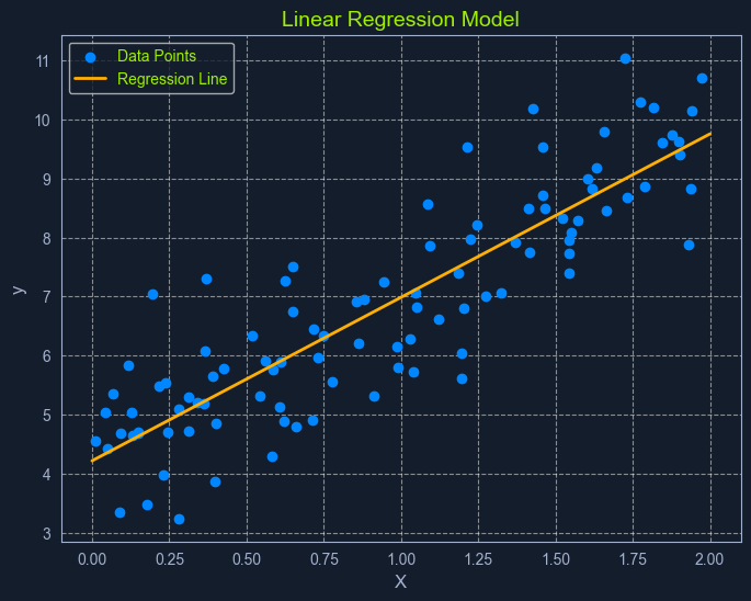
Linear Regression is a fundamental supervised learning algorithm that predicts a continuous target variable by establishing a linear relationship between the target and one or more predictor variables. The algorithm models this relationship using a linear equation, where changes in the predictor variables result in proportional changes in the target variable. The goal is to find the best-fitting line that minimizes the sum of the squared differences between the predicted values and the actual values.
Imagine you're trying to predict a house's price based on size. Linear regression would attempt to find a straight line that best captures the relationship between these two variables. As the size of the house increases, the price generally tends to increase. Linear regression quantifies this relationship, allowing us to predict the price of a house given its size.
Before diving into linear regression, it's essential to understand the broader concept of regression in machine learning. Regression analysis is a type of supervised learning where the goal is to predict a continuous target variable. This target variable can take on any value within a given range. Think of it as estimating a number instead of classifying something into categories (which is what classification algorithms do).
Examples of regression problems include:
In all these cases, the output we're trying to predict is a continuous value. This is what distinguishes regression from classification, where the output is a categorical label (e.g., "spam" or "not spam").
Now, with that clarified, let's revisit linear regression. It's simply one specific type of regression analysis where we assume a linear relationship between the predictor variables and the target variable. This means we try to model the relationship using a straight line.
In its simplest form, simple linear regression involves one predictor variable and one target variable. A linear equation represents the relationship between them:
Code: python
y = mx + c
Where:
y is the predicted target variablex is the predictor variablem is the slope of the line (representing the relationship between x and y)c is the y-intercept (the value of y when x is 0)The algorithm aims to find the optimal values for m and c that minimize the error between the predicted y values and the actual y values in the training data. This is typically done using Ordinary Least Squares (OLS), which aims to minimize the sum of squared errors.
When multiple predictor variables are involved, it's called multiple linear regression. The equation becomes:
Code: python
y = b0 + b1x1 + b2x2 + ... + bnxn
Where:
y is the predicted target variablex1, x2, ..., xn are the predictor variablesb0 is the y-interceptb1, b2, ..., bn are the coefficients representing the relationship between each predictor variable and the target variable.
Ordinary Least Squares (OLS) is a common method for estimating the optimal values for the coefficients in linear regression. It aims to minimize the sum of the squared differences between the actual values and the values predicted by the model.
Think of it as finding the line that minimizes the total area of the squares formed between the data points and the line. This "line of best fit" represents the relationship that best describes the data.
Here's a breakdown of the OLS process:
Calculate Residuals: For each data point, the residual is the difference between the actual y value and the y value predicted by the model.Square the Residuals: Each residual is squared to ensure that all values are positive and to give more weight to larger errors.Sum the Squared Residuals: All the squared residuals are summed to get a single value representing the model's overall error. This sum is called the Residual Sum of Squares (RSS).Minimize the Sum of Squared Residuals: The algorithm adjusts the coefficients to find the values that result in the smallest possible RSS.This process can be visualized as finding the line that minimizes the total area of the squares formed between the data points and the line.
Linear regression relies on several key assumptions about the data:
Linearity: A linear relationship exists between the predictor and target variables.Independence: The observations in the dataset are independent of each other.Homoscedasticity: The variance of the errors is constant across all levels of the predictor variables. This means the spread of the residuals should be roughly the same across the range of predicted values.Normality: The errors are normally distributed. This assumption is important for making valid inferences about the model's coefficients.Assessing these assumptions before applying linear regression ensures the model's validity and reliability. If these assumptions are violated, the model's predictions may be inaccurate or misleading.
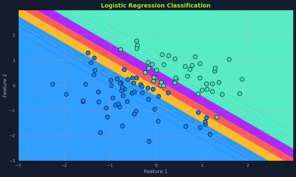
Despite its name, logistic regression is a supervised learning algorithm primarily used for classification, not regression. It predicts a categorical target variable with two possible outcomes (binary classification). These outcomes are typically represented as binary values (e.g., 0 or 1, true or false, yes or no).
For example, logistic regression can predict whether an email is spam or not or whether a customer will click on an ad. The algorithm models the probability of the target variable belonging to a particular class using a logistic function, which maps the input features to a value between 0 and 1.
Before we delve deeper into logistic regression, let's clarify what classification means in machine learning. Classification is a type of supervised learning that aims to assign data points to specific categories or classes. Unlike regression, which predicts a continuous value, classification predicts a discrete label.
Examples of classification problems include:
In all these cases, the output we're trying to predict is a category or class label.
Unlike linear regression, which outputs a continuous value, logistic regression outputs a probability score between 0 and 1. This score represents the likelihood of the input belonging to the positive class (typically denoted as '1').
It achieves this by employing a sigmoid function, which maps any input value (a linear combination of features) to a value within the 0 to 1 range. This function introduces non-linearity, allowing the model to capture complex relationships between the features and the probability of the outcome.
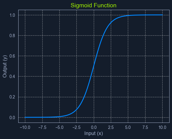
The sigmoid function is a mathematical function that takes any input value (ranging from negative to positive infinity) and maps it to an output value between 0 and 1. This makes it particularly useful for modeling probabilities.
The sigmoid function has a characteristic "S" shape, hence its name. It starts with low values for negative inputs, then rapidly increases around zero, and finally plateaus at high values for positive ones. This smooth, gradual transition between 0 and 1 allows it to represent the probability of an event occurring.
In logistic regression, the sigmoid function transforms the linear combination of input features into a probability score. This score represents the likelihood of the input belonging to the positive class.
The sigmoid function's mathematical representation is:
Code: python
P(x) = 1 / (1 + e^-z)
Where:
P(x) is the predicted probability.e is the base of the natural logarithm (approximately 2.718).z is the linear combination of input features and their weights, similar to the linear regression equation: z = m1x1 + m2x2 + ... + mnxn + cLet's say we're building a spam filter using logistic regression. The algorithm would analyze various email features, such as the sender's address, the presence of certain keywords, and the email's content, to calculate a probability score. The email will be classified as spam if the score exceeds a predefined threshold (e.g., 0.8).
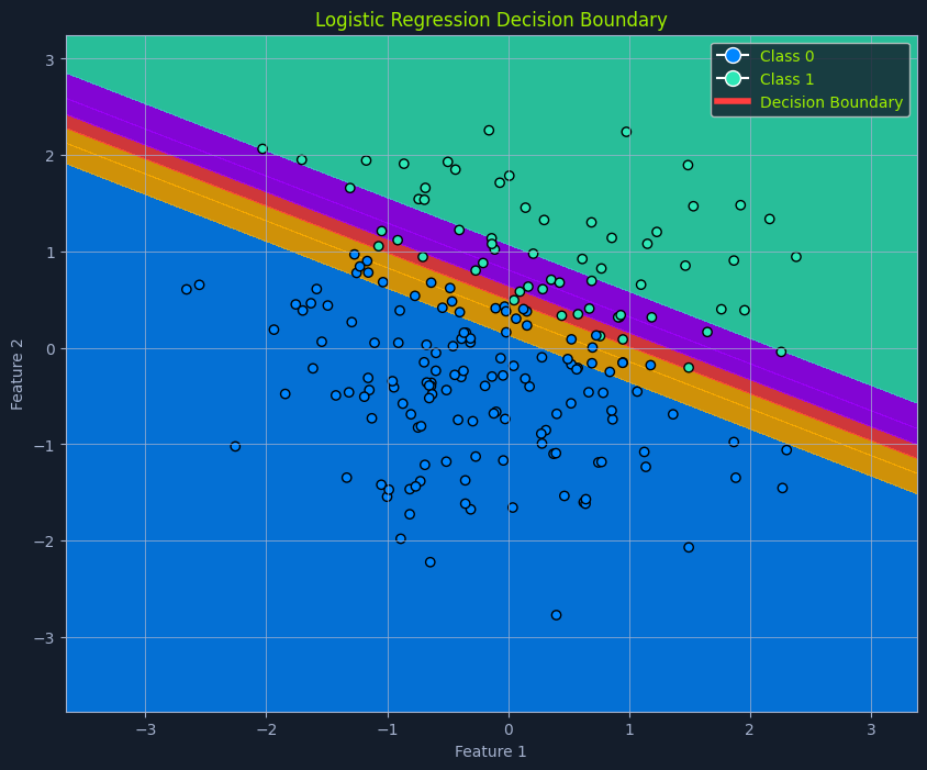
A crucial aspect of logistic regression is the decision boundary. In a simplified scenario with two features, imagine a line separating the data points into two classes. This separator is the decision boundary, determined by the model's learned parameters and the chosen threshold probability.
In higher dimensions with more features, this separator becomes a hyperplane. The decision boundary defines the cutoff point for classifying an instance into one class or another.

In the context of machine learning, a hyperplane is a subspace whose dimension is one less than that of the ambient space. It's a way to visualize a decision boundary in higher dimensions.
Think of it this way:
Moving to higher dimensions (with more than three features) makes it difficult to visualize, but the concept remains the same. A hyperplane is a "flat" subspace that divides the higher-dimensional space into two regions.
In logistic regression, the hyperplane is defined by the model's learned parameters (coefficients) and the chosen threshold probability. It acts as the decision boundary, separating data points into classes based on their predicted probabilities.
The threshold probability is often set at 0.5 but can be adjusted depending on the specific problem and the desired balance between true and false positives.
P(x) falls above the threshold, the instance is classified as the positive class.P(x) falls below the threshold, it's classified as the negative class.For example, in spam detection, if the model predicts an email has a 0.8 probability of being spam (and the threshold is 0.5), it's classified as spam. Adjusting the threshold to 0.6 would require a higher probability for the email to be classified as spam.
While not as strict as linear regression, logistic regression does have some underlying assumptions about the data:
Binary Outcome: The target variable must be categorical, with only two possible outcomes.Linearity of Log Odds: It assumes a linear relationship between the predictor variables and the log-odds of the outcome. Log odds are a transformation of probability, representing the logarithm of the odds ratio (the probability of an event occurring divided by the probability of it not occurring).No or Little Multicollinearity: Ideally, there should be little to no multicollinearity among the predictor variables. Multicollinearity occurs when predictor variables are highly correlated, making it difficult to determine their individual effects on the outcome.Large Sample Size: Logistic regression performs better with larger datasets, allowing for more reliable parameter estimation.Assessing these assumptions before applying logistic regression helps ensure the model's accuracy and reliability. Techniques like data exploration, visualization, and statistical tests can be used to evaluate these assumptions.
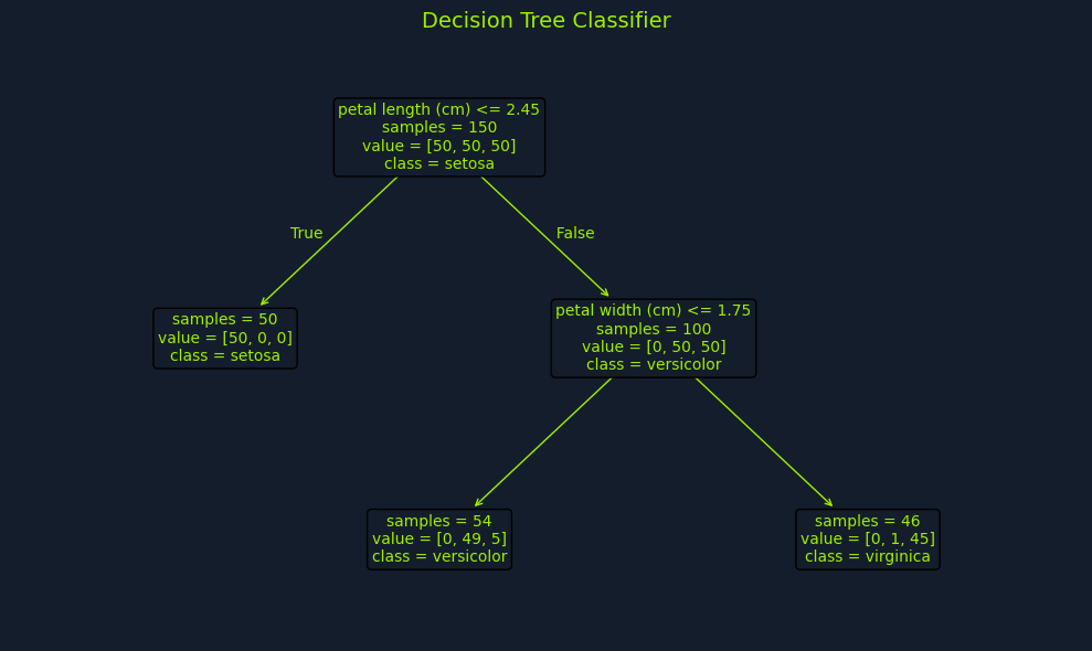
Decision trees are a popular supervised learning algorithm for classification and regression tasks. They are known for their intuitive tree-like structure, which makes them easy to understand and interpret. In essence, a decision tree creates a model that predicts the value of a target variable by learning simple decision rules inferred from the data features.
Imagine you're trying to decide whether to play tennis based on the weather. A decision tree would break down this decision into a series of simple questions: Is it sunny? Is it windy? Is it humid? Based on the answers to these questions, the tree would lead you to a final decision: play tennis or don't play tennis.
A decision tree comprises three main components:
Root Node: This represents the starting point of the tree and contains the entire dataset.Internal Nodes: These nodes represent features or attributes of the data. Each internal node branches into two or more child nodes based on different decision rules.Leaf Nodes: These are the terminal nodes of the tree, representing the final outcome or prediction.Building a decision tree involves selecting the best feature to split the data at each node. This selection is based on measures like Gini impurity, entropy, or information gain, which quantify the homogeneity of the subsets resulting from the split. The goal is to create splits that result in increasingly pure subsets, where the data points within each subset belong predominantly to the same class.
Gini impurity measures the probability of misclassifying a randomly chosen element from a set. A lower Gini impurity indicates a more pure set. The formula for Gini impurity is:
Gini(S) = 1 - Σ (pi)^2
Where:
S is the dataset.pi is the proportion of elements belonging to class i in the set.Consider a dataset S with two classes: A and B. Suppose there are 30 instances of class A and 20 instances of class B in the dataset.
A: pA = 30 / (30 + 20) = 0.6B: pB = 20 / (30 + 20) = 0.4The Gini impurity for this dataset is:
Gini(S) = 1 - (0.6^2 + 0.4^2) = 1 - (0.36 + 0.16) = 1 - 0.52 = 0.48
Entropy measures the disorder or uncertainty in a set. A lower entropy indicates a more homogenous set. The formula for entropy is:
Entropy(S) = - Σ pi * log2(pi)
Where:
S is the dataset.pi is the proportion of elements belonging to class i in the set.Using the same dataset S with 30 instances of class A and 20 instances of class B:
A: pA = 0.6B: pB = 0.4The entropy for this dataset is:
Entropy(S) = - (0.6 * log2(0.6) + 0.4 * log2(0.4))
           = - (0.6 * (-0.73697) + 0.4 * (-1.32193))
           = - (-0.442182 - 0.528772)
           = 0.970954
Information gain measures the reduction in entropy achieved by splitting a set based on a particular feature. The feature with the highest information gain is chosen for the split. The formula for information gain is:
Information Gain(S, A) = Entropy(S) - Σ ((|Sv| / |S|) * Entropy(Sv))
Where:
S is the dataset.A is the feature used for splitting.Sv is the subset of S for which feature A has value v.Consider a dataset S with 50 instances and two classes: A and B. Suppose we consider a feature F that can take on two values: 1 and 2. The distribution of the dataset is as follows:
F = 1: 30 instances, 20 class A, 10 class BF = 2: 20 instances, 10 class A, 10 class BFirst, calculate the entropy of the entire dataset S:
Entropy(S) = - (30/50 * log2(30/50) + 20/50 * log2(20/50))
           = - (0.6 * log2(0.6) + 0.4 * log2(0.4))
           = - (0.6 * (-0.73697) + 0.4 * (-1.32193))
           = 0.970954
Next, calculate the entropy for each subset Sv:
F = 1:A: pA = 20/30 = 0.6667B: pB = 10/30 = 0.3333- (0.6667 * log2(0.6667) + 0.3333 * log2(0.3333)) = 0.9183F = 2:A: pA = 10/20 = 0.5B: pB = 10/20 = 0.5- (0.5 * log2(0.5) + 0.5 * log2(0.5)) = 1.0Now, calculate the weighted average entropy of the subsets:
Weighted Entropy = (|S1| / |S|) * Entropy(S1) + (|S2| / |S|) * Entropy(S2)
                 = (30/50) * 0.9183 + (20/50) * 1.0
                 = 0.55098 + 0.4
                 = 0.95098
Finally, calculate the information gain:
Information Gain(S, F) = Entropy(S) - Weighted Entropy
                       = 0.970954 - 0.95098
                       = 0.019974
The tree starts with the root node and selects the feature that best splits the data based on one of these criteria (Gini impurity, entropy, or information gain). This feature becomes the internal node, and branches are created for each possible value or range of values of that feature. The data is then divided into subsets based on these branches. This process continues recursively for each subset until a stopping criterion is met.
The tree stops growing when one of the following conditions is satisfied:
Maximum Depth : The tree reaches a specified maximum depth, preventing it from becoming overly complex and potentially overfitting the data.Minimum Number of Data Points : The number of data points in a node falls below a specified threshold, ensuring that the splits are meaningful and not based on very small subsets.Pure Nodes : All data points in a node belong to the same class, indicating that further splits would not improve the purity of the subsets.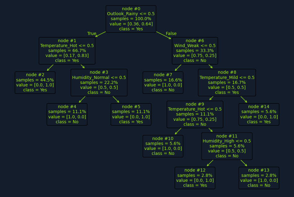
Let's examine the "Playing Tennis" example more closely to illustrate how a decision tree works in practice.
Imagine you have a dataset of historical weather conditions and whether you played tennis on those days. For example:
| PlayTennis | Outlook_Overcast | Outlook_Rainy | Outlook_Sunny | Temperature_Cool | Temperature_Hot | Temperature_Mild | Humidity_High | Humidity_Normal | Wind_Strong | Wind_Weak |
|---|---|---|---|---|---|---|---|---|---|---|
| No | False | True | False | True | False | False | False | True | False | True |
| Yes | False | False | True | False | True | False | False | True | False | True |
| No | False | True | False | True | False | False | True | False | True | False |
| No | False | True | False | False | True | False | True | False | False | True |
| Yes | False | False | True | False | False | True | False | True | False | True |
| Yes | False | False | True | False | True | False | False | True | False | True |
| No | False | True | False | False | True | False | True | False | True | False |
| Yes | True | False | False | True | False | False | True | False | False | True |
| No | False | True | False | False | True | False | False | True | True | False |
| No | False | True | False | False | True | False | True | False | True | False |
The dataset includes the following features:
Outlook: Sunny, Overcast, RainyTemperature: Hot, Mild, CoolHumidity: High, NormalWind: Weak, StrongThe target variable is Play Tennis: Yes or No.
A decision tree algorithm would analyze this dataset to identify the features that best separate the "Yes" instances from the "No" instances. It would start by calculating each feature's information gain or Gini impurity to determine which provides the most informative split.
For instance, the algorithm might find that the Outlook feature provides the highest information gain. This means splitting the data based on whether sunny, overcast, or rainy leads to the most significant reduction in entropy or impurity.
The root node of the decision tree would then be the Outlook feature, with three branches: Sunny, Overcast, and Rainy. Based on these branches, the dataset would be divided into three subsets.
Next, the algorithm would analyze each subset to determine the best feature for the next split. For example, in the "Sunny" subset, Humidity might provide the highest information gain. This would lead to another internal node with High and Normal branches.
This process continues recursively until a stopping criterion is met, such as reaching a maximum depth or a minimum number of data points in a node. The final result is a tree-like structure with decision rules at each internal node and predictions (Play Tennis: Yes or No) at the leaf nodes.
One of the advantages of decision trees is that they have minimal assumptions about the data:
No Linearity Assumption: Decision trees can handle linear and non-linear relationships between features and the target variable. This makes them more flexible than algorithms like linear regression, which assume a linear relationship.No Normality Assumption: The data does not need to be normally distributed. This contrasts some statistical methods that require normality for valid inferences.Handles Outliers: Decision trees are relatively robust to outliers. Since they partition the data based on feature values rather than relying on distance-based calculations, outliers are less likely to have a significant impact on the tree structure.These minimal assumptions contribute to decision trees' versatility, allowing them to be applied to a wide range of datasets and problems without extensive preprocessing or transformations.
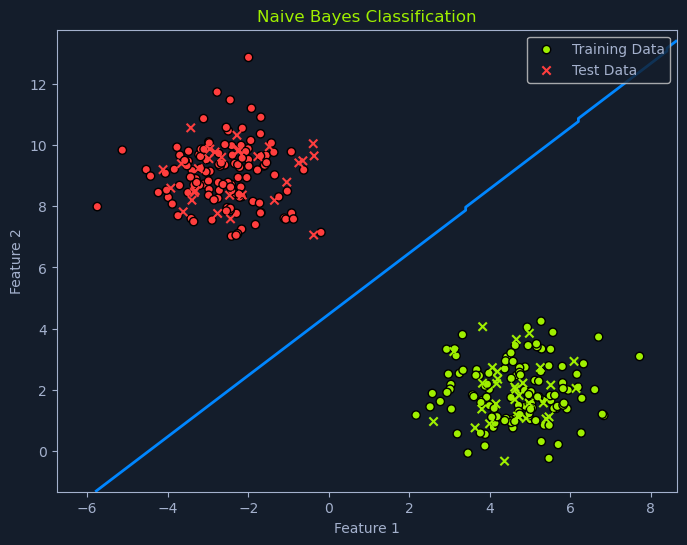
Naive Bayes is a probabilistic algorithm used for classification tasks. It's based on Bayes' theorem, a fundamental concept in probability theory that describes the probability of an event based on prior knowledge and observed evidence. Naive Bayes is a popular choice for tasks like spam filtering and sentiment analysis due to its simplicity, efficiency, and surprisingly good performance in many real-world scenarios.
Before diving into Naive Bayes, let's understand its core concept: Bayes' theorem. This theorem provides a way to update our beliefs about an event based on new evidence. It allows us to calculate the probability of an event, given that another event has already occurred.
It's mathematically represented as:
Code: python
P(A|B) = [P(B|A) * P(A)] / P(B)
Where:
P(A|B): The posterior probability of event A happening, given that event B has already happened.P(B|A): The likelihood of event B happening given that event A has already happened.P(A): The prior probability of event A happening.P(B): The prior probability of event B happening.Let's say we want to know the probability of someone having a disease (A) given that they tested positive for it (B). Bayes' theorem allows us to calculate this probability using the prior probability of having the disease (P(A)), the likelihood of testing positive given that the person has the disease (P(B|A)), and the overall probability of testing positive (P(B)).
Suppose we have the following information:
P(A) = 0.01.P(B|A) = 0.95.P(B), can be calculated using the law of total probability.First, let's calculate P(B):
Code: python
P(B) = P(B|A) * P(A) + P(B|¬A) * P(¬A)
Where:
P(¬A): The probability of not having the disease, which is 1 - P(A) = 0.99.P(B|¬A): The probability of testing positive given that the person does not have the disease, which is the false positive rate, 0.05.Now, substitute the values:
Code: python
P(B) = (0.95 * 0.01) + (0.05 * 0.99)
     = 0.0095 + 0.0495
     = 0.059
Next, we use Bayes' theorem to find P(A|B):
Code: python
P(A|B) = [P(B|A) * P(A)] / P(B)
        = (0.95 * 0.01) / 0.059
        = 0.0095 / 0.059
        ≈ 0.161
So, the probability of someone having the disease, given that they tested positive, is approximately 16.1%.
This example demonstrates how Bayes' theorem can be used to update our beliefs about the likelihood of an event based on new evidence. In this case, even though the test is quite accurate, the low prevalence of the disease means that a positive test result still has a relatively low probability of indicating the actual presence of the disease.
The Naive Bayes classifier leverages Bayes' theorem to predict the probability of a data point belonging to a particular class given its features. To do this, it makes the "naive" assumption of conditional independence among the features. This means it assumes that the presence or absence of one feature doesn't affect the presence or absence of any other feature, given that we know the class label.
Let's break down how this works in practice:
Calculate Prior Probabilities: The algorithm first calculates the prior probability of each class. This is the probability of a data point belonging to a particular class before considering its features. For example, in a spam detection scenario, the probability of an email being spam might be 0.2 (20%), while the probability of it being not spam is 0.8 (80%).Calculate Likelihoods: Next, the algorithm calculates the likelihood of observing each feature given each class. This involves determining the probability of seeing a particular feature value given that the data point belongs to a specific class. For instance, what's the likelihood of seeing the word "free" in an email given that it's spam? What's the likelihood of seeing the word "meeting" given that it's not spam?Apply Bayes' Theorem: For a new data point, the algorithm combines the prior probabilities and likelihoods using Bayes' theorem to calculate the posterior probability of the data point belonging to each class. The posterior probability is the updated probability of an event (in this case, the data point belonging to a certain class) after considering new information (the observed features). This represents the revised belief about the class label after considering the observed features.Predict the Class: Finally, the algorithm assigns the data point to the class with the highest posterior probability.While this assumption of feature independence is often violated in real-world data (words like "free" and "viagra" might indeed co-occur more often in spam), Naive Bayes often performs surprisingly well in practice.
The specific implementation of Naive Bayes depends on the type of features and their assumed distribution:
Gaussian Naive Bayes: This is used when the features are continuous and assumed to follow a Gaussian distribution (a bell curve). For example, if predicting whether a customer will purchase a product based on their age and income, Gaussian Naive Bayes could be used, assuming age and income are normally distributed.Multinomial Naive Bayes: This is suitable for discrete features and is often used in text classification. For instance, in spam filtering, the frequency of words like "free" or "money" might be the features, and Multinomial Naive Bayes would model the probability of these words appearing in spam and non-spam emails.Bernoulli Naive Bayes: This type is employed for binary features, where the feature is either present or absent. In document classification, a feature could be whether a specific word is present in the document. Bernoulli Naive Bayes would model the probability of this presence or absence for each class.The choice of which type of Naive Bayes to use depends on the nature of the data and the specific problem being addressed.
While Naive Bayes is relatively robust, it's helpful to be aware of some data assumptions:
Feature Independence: As discussed, the core assumption is that features are conditionally independent given the class.Data Distribution: The choice of Naive Bayes classifier (Gaussian, Multinomial, Bernoulli) depends on the assumed distribution of the features.Sufficient Training Data: Although Naive Bayes can work with limited data, it is important to have sufficient data to estimate probabilities accurately.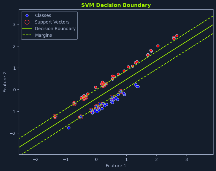
Support Vector Machines (SVMs) are powerful supervised learning algorithms for classification and regression tasks. They are particularly effective in handling high-dimensional data and complex non-linear relationships between features and the target variable. SVMs aim to find the optimal hyperplane that maximally separates different classes or fits the data for regression.
An SVM aims to find the hyperplane that maximizes the margin. The margin is the distance between the hyperplane and the nearest data points of each class. These nearest data points are called support vectors and are crucial in defining the hyperplane and the margin.
By maximizing the margin, SVMs aim to find a robust decision boundary that generalizes well to new, unseen data. A larger margin provides more separation between the classes, reducing the risk of misclassification.
A linear SVM is used when the data is linearly separable, meaning a straight line or hyperplane can perfectly separate the classes. The goal is to find the optimal hyperplane that maximizes the margin while correctly classifying all the training data points.
Imagine you're tasked with classifying emails as spam or not spam based on the frequency of the words "free" and "money." If we plot each email on a graph where the x-axis represents the frequency of "free" and the y-axis represents the frequency of "money," we can visualize how SVMs work.
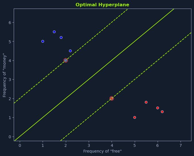
The optimal hyperplane is the one that maximizes the margin between the closest data points of different classes. This margin is called the separating hyperplane. The data points closest to the hyperplane are called support vectors, as they "support" or define the hyperplane and the margin.
Maximizing the margin is intended to create a robust classifier. A larger margin allows the SVM to tolerate some noise or variability in the data without misclassifying points. It also improves the model's generalization ability, making it more likely to perform well on unseen data.
In the spam classification scenario depicted in the graph, the linear SVM identifies the line that maximizes the distance between the nearest spam and non-spam emails. This line serves as the decision boundary for classifying new emails. Emails falling on one side of the line are classified as spam, while those on the other side are classified as not spam.
The hyperplane is defined by an equation of the form:
Code: python
w * x + b = 0
Where:
w is the weight vector, perpendicular to the hyperplane.x is the input feature vector.b is the bias term, which shifts the hyperplane relative to the origin.The SVM algorithm learns the optimal values for w and b during the training process.

In many real-world scenarios, data is not linearly separable. This means we cannot draw a straight line or hyperplane to perfectly separate the different classes. In these cases, non-linear SVMs come to the rescue.
Non-linear SVMs utilize a technique called the kernel trick. This involves using a kernel function to map the original data points into a higher-dimensional space where they become linearly separable.
Imagine separating a mixture of red and blue marbles on a table. If the marbles are mixed in a complex pattern, you might be unable to draw a straight line to separate them. However, if you could lift some marbles off the table (into a higher dimension), you might be able to find a plane that separates them.
This is essentially what a kernel function does. It transforms the data into a higher-dimensional space where a linear hyperplane can be found. This hyperplane corresponds to a non-linear decision boundary when mapped back to the original space.
Several kernel functions are commonly used in non-linear SVMs:
Polynomial Kernel: This kernel introduces polynomial terms (like x², x³, etc.) to capture non-linear relationships between features. It's like adding curves to the decision boundary.Radial Basis Function (RBF) Kernel: This kernel uses a Gaussian function to map data points to a higher-dimensional space. It's one of the most popular and versatile kernel functions, capable of capturing complex non-linear patterns.Sigmoid Kernel: This kernel is similar to the sigmoid function used in logistic regression. It introduces non-linearity by mapping the data points to a space with a sigmoid-shaped decision boundary.The kernel function choice depends on the data's nature and the model's desired complexity.
Non-linear SVMs are particularly useful in applications like image classification. Images often have complex patterns that linear boundaries cannot separate.
For instance, imagine classifying images of cats and dogs. The features might be things like fur texture, ear shape, and facial features. These features often have non-linear relationships. A non-linear SVM with an appropriate kernel function can capture these relationships and effectively separate cat images from dog images.
Finding this optimal hyperplane involves solving an optimization problem. The problem can be formulated as:
Code: python
Minimize: 1/2 ||w||^2
Subject to: yi(w * xi + b) >= 1 for all i
Where:
w is the weight vector that defines the hyperplanexi is the feature vector for data point iyi is the class label for data point i (-1 or 1)b is the bias termThis formulation aims to minimize the magnitude of the weight vector (which maximizes the margin) while ensuring that all data points are correctly classified with a margin of at least 1.
SVMs have few assumptions about the data:
No Distributional Assumptions: SVMs do not make strong assumptions about the underlying distribution of the data.Handles High Dimensionality: They are effective in high-dimensional spaces, where the number of features is larger than the number of data points.Robust to Outliers: SVMs are relatively robust to outliers, focusing on maximizing the margin rather than fitting all data points perfectly.SVMs are powerful and versatile algorithms that have proven effective in various machine-learning tasks. Their ability to handle high-dimensional data and complex non-linear relationships makes them a valuable tool for solving challenging classification and regression problems.
Unsupervised learning algorithms explore unlabeled data, where the goal is not to predict a specific outcome but to discover hidden patterns, structures, and relationships within the data. Unlike supervised learning, where the algorithm learns from labeled examples, unsupervised learning operates without the guidance of predefined labels or "correct answers."
Think of it as exploring a new city without a map. You observe the surroundings, identify landmarks, and notice how different areas are connected. Similarly, unsupervised learning algorithms analyze the inherent characteristics of the data to uncover hidden structures and patterns.
Unsupervised learning algorithms identify similarities, differences, and patterns in the data. They can group similar data points together, reduce the number of variables while preserving essential information, or identify unusual data points that deviate from the norm.
These algorithms are valuable for tasks where labeled data is scarce, expensive, or unavailable. They enable us to gain insights into the data's underlying structure and organization, even without knowing the specific outcomes or labels.
Unsupervised learning problems can be broadly categorized into:
Clustering: Grouping similar data points together based on their characteristics. This is like organizing a collection of books by genre or grouping customers based on their purchasing behavior.Dimensionality Reduction: Reducing the number of variables (features) in the data while preserving essential information. This is analogous to summarizing a long document into a concise abstract or compressing an image without losing its important details.Anomaly Detection: Identifying unusual data points that deviate significantly from the norm. This is like spotting a counterfeit bill among a stack of genuine ones or detecting fraudulent credit card transactions.To effectively understand unsupervised learning, it's crucial to grasp some core concepts.
The cornerstone of unsupervised learning is unlabeled data. Unlike supervised learning, where data points come with corresponding labels or target variables, unlabeled data lacks these predefined outcomes. The algorithm must rely solely on the data's inherent characteristics and input features to discover patterns and relationships.
Think of it as analyzing a collection of photographs without any captions or descriptions. Even without knowing the specific context of each photo, you can still group similar photos based on visual features like color, composition, and subject matter.
Many unsupervised learning algorithms rely on quantifying the similarity or dissimilarity between data points. Similarity measures calculate how alike or different two data points are based on their features. Common measures include:
Euclidean Distance: Measures the straight-line distance between two points in a multi-dimensional space.Cosine Similarity: Measures the angle between two vectors, representing data points, with higher values indicating greater similarity.Manhattan Distance: Calculates the distance between two points by summing the absolute differences of their coordinates.The choice of similarity measure depends on the nature of the data and the specific algorithm being used.
Clustering tendency refers to the data's inherent propensity to form clusters or groups. Before applying clustering algorithms, assessing whether the data exhibits a natural tendency to form clusters is essential. If the data is uniformly distributed without inherent groupings, clustering algorithms might not yield meaningful results.
Evaluating the quality and meaningfulness of the clusters produced by a clustering algorithm is crucial. Cluster validity involves assessing metrics like:
Cohesion: Measures how similar data points are within a cluster. Higher cohesion indicates a more compact and well-defined cluster.Separation: Measures how different clusters are from each other. Higher separation indicates more distinct and well-separated clusters.Various cluster validity indices, such as the silhouette score and Davies-Bouldin index, quantify these aspects and help determine the optimal number of clusters.
Dimensionality refers to the number of features or variables in the data. High dimensionality can pose challenges for some unsupervised learning algorithms, increasing computational complexity and potentially leading to the "curse of dimensionality," where data becomes sparse and distances between points become less meaningful.
The intrinsic dimensionality of data represents its inherent or underlying dimensionality, which may be lower than the actual number of features. It captures the essential information contained in the data. Dimensionality reduction techniques aim to reduce the number of features while preserving this intrinsic dimensionality.
An anomaly is a data point that deviates significantly from the norm or expected pattern in the data. Anomalies can represent unusual events, errors, or fraudulent activities. Detecting anomalies is crucial in various applications, such as fraud detection, network security, and system monitoring.
An outlier is a data point that is far away from the majority of other data points. While similar to an anomaly, the term "outlier" is often used in a broader sense. Outliers can indicate errors in data collection, unusual observations, or potentially interesting patterns.
Feature scaling is essential in unsupervised learning to ensure that all features contribute equally to the distance calculations and other computations. Common techniques include:
Min-Max Scaling: Scales features to a fixed range.Standardization (Z-score normalization): Transforms features to have zero mean and unit variance.
K-means clustering is a popular unsupervised learning algorithm for partitioning a dataset into K distinct, non-overlapping clusters. The goal is to group similar data points, where similarity is typically measured by the distance between data points in a multi-dimensional space.
Imagine you have a dataset of customers with information about their purchase history, demographics, and browsing activity. K-means clustering can group these customers into distinct segments based on their similarities. This can be valuable for targeted marketing, personalized recommendations, and customer relationship management.
K-means is an iterative algorithm that aims to minimize the variance within each cluster. This means it tries to group data points so that the points within a cluster are as close to each other and as far from data points in other clusters as possible.
The algorithm follows these steps:
Initialization: Randomly select K data points from the dataset as the initial cluster centers (centroids). These centroids represent the average point within each cluster.Assignment: Assign each data point to the nearest cluster center based on a distance metric, such as Euclidean distance.Update: Recalculate the cluster centers by taking the mean of all data points assigned to each cluster. This updates the centroid to represent the center of the cluster better.Iteration: Repeat steps 2 and 3 until the cluster centers no longer change significantly or a maximum number of iterations is reached. This iterative process refines the clusters until they stabilize.Euclidean distance is a common distance metric used to measure the similarity between data points in K-means clustering. It calculates the straight-line distance between two points in a multi-dimensional space.
For two data points x and y with n features, the Euclidean distance is calculated as:
Code: python
d(x, y) = sqrt(Σ (xi - yi)^2)
Where:
xi and yi are the values of the i-th feature for data points x and y, respectively.Determining the optimal number of clusters (K) is crucial in K-means clustering. The choice of K significantly impacts the clustering results and their interpretability. Selecting too few clusters can lead to overly broad groupings, while selecting too many can result in overly granular and potentially meaningless clusters.
Unfortunately, there is no one-size-fits-all method for determining the optimal K. It often involves a combination of techniques and domain expertise.
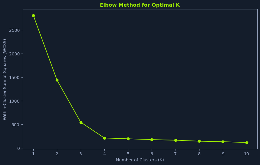
The Elbow Method is a graphical technique that helps estimate the optimal K by visualizing the relationship between the number of clusters and the within-cluster sum of squares (WCSS).
It follows the following steps:
Run K-means for a range of K values: Perform K-means clustering for different values of K, typically starting from 1 and increasing incrementally.Calculate WCSS: For each value of K, calculate the WCSS. The WCSS measures the total variance within each cluster. Lower WCSS values indicate that the data points within clusters are more similar.Plot WCSS vs. K: Plot the WCSS values against the corresponding K values.Identify the Elbow Point: Look for the "elbow" point in the plot. This is where the WCSS starts to decrease at a slower rate. This point often suggests a good value for K, indicating a balance between minimizing within-cluster variance and avoiding excessive granularity.The elbow point represents a trade-off between model complexity and model fit. Increasing K beyond the elbow point might lead to overfitting, where the model captures noise in the data rather than meaningful patterns.
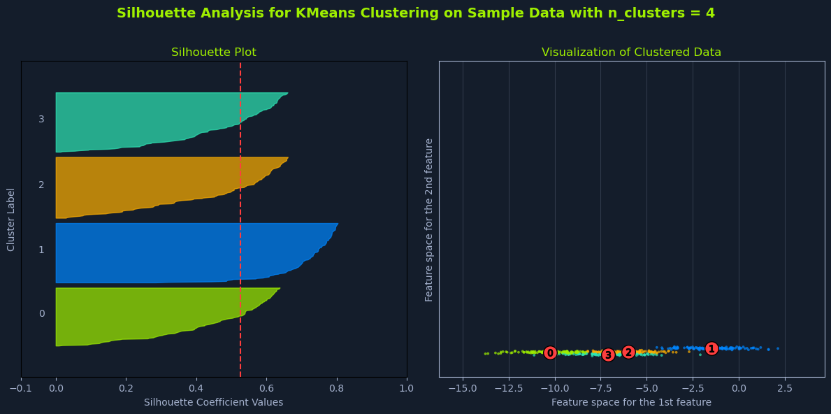
Silhouette analysis provides a more quantitative approach to evaluating different values of K. It measures how similar a data point is to its own cluster compared to others.
The process is broken down into four core steps:
Run K-means for a range of K values: Similar to the elbow method, perform K-means clustering for different values of K.Calculate Silhouette Scores: For each data point, calculate its silhouette score. The silhouette score ranges from -1 to 1, where:Calculate Average Silhouette Score: For each value of K, calculate the average silhouette score across all data points.Choose K with the Highest Score: Select the value of K that yields the highest average silhouette score. This indicates the clustering solution with the best-defined clusters.Higher silhouette scores generally indicate better-defined clusters, where data points are more similar to their cluster and less similar to others.
While the elbow method and silhouette analysis provide valuable guidance, domain expertise is often crucial in choosing the optimal K. Consider the problem's specific context and the desired level of granularity in the clusters.
In some cases, practical considerations might outweigh purely quantitative measures. For instance, if the goal is to segment customers for targeted marketing, you might choose a K that aligns with the number of distinct marketing campaigns you can realistically manage.
Other factors to consider include:
Computational Cost: Higher values of K generally require more computational resources.Interpretability: The resulting clusters should be meaningful and interpretable in the context of the problem.By combining these techniques and considering the task's specific requirements, you can effectively choose an optimal K for K-means clustering that yields meaningful and insightful results.
K-means clustering makes certain assumptions about the data:
Cluster Shape: It assumes that clusters are spherical and have similar sizes. This means it might not perform well if the clusters have complex shapes or vary significantly in size.Feature Scale: It is sensitive to the scale of the features. Features with larger scales can have a greater influence on the clustering results. Therefore, it's important to standardize or normalize the data before applying K-means.Outliers: K-means can be sensitive to outliers, data points that deviate significantly from the norm. Outliers can distort the cluster centers and affect the clustering results.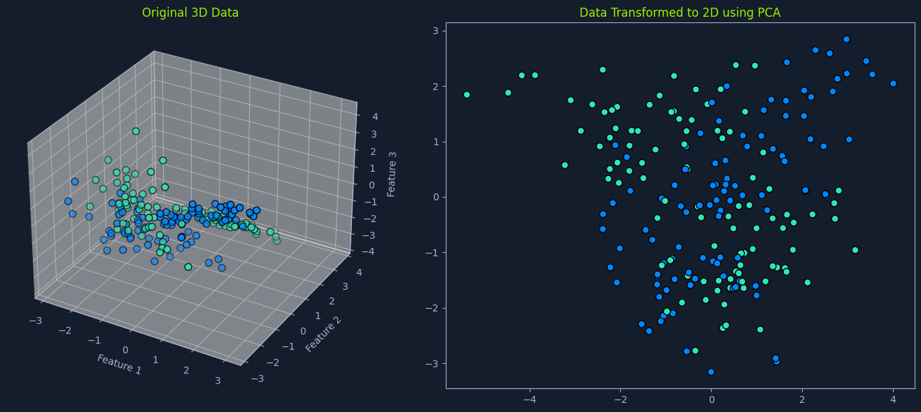
Principal Component Analysis (PCA) is a dimensionality reduction technique that transforms high-dimensional data into a lower-dimensional representation while preserving as much original information as possible. It achieves this by identifying the principal components and new variables that are linear combinations of the original features and capturing the maximum variance in the data. PCA is widely used for feature extraction, data visualization, and noise reduction.
For example, in image processing, PCA can reduce the dimensionality of image data by identifying the principal components that capture the most important features of the images, such as edges, textures, and shapes.
Think of it as finding the most important "directions" in the data. Imagine a scatter plot of data points. PCA finds the lines that best capture the spread of the data. These lines represent the principal components.
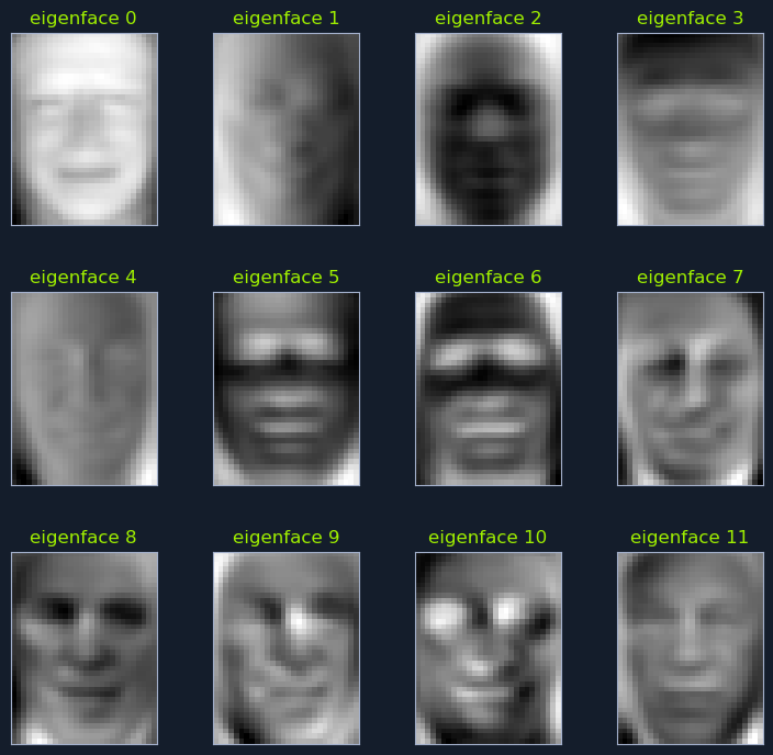
Consider a database of facial images. PCA can be used to identify the principal components that capture the most significant variations in facial features, such as eye shape, nose size, and mouth width. By projecting the facial images onto a lower-dimensional space defined by these principal components, we can efficiently search for similar faces.
There are three key concepts to PCA:
Variance: Variance measures the spread or dispersion of data points around the mean. PCA aims to find principal components that maximize variance, capturing the most significant information in the data.Covariance: Covariance measures the relationship between two variables. PCA considers the covariance between different features to identify the directions of maximum variance.Eigenvectors and Eigenvalues: Eigenvectors represent the directions of the principal components, and eigenvalues represent the amount of variance explained by each principal component.The PCA algorithm follows these steps:
Standardize the data: Subtract the mean and divide by the standard deviation for each feature to ensure that all features have the same scale.Calculate the covariance matrix: Compute the covariance matrix of the standardized data, which represents the relationships between different features.Compute the eigenvectors and eigenvalues: Determine the eigenvectors and eigenvalues of the covariance matrix. The eigenvectors represent the directions of the principal components, and the eigenvalues represent the amount of variance explained by each principal component.Sort the eigenvectors: Sort the eigenvectors in descending order of their corresponding eigenvalues. The eigenvectors with the highest eigenvalues capture the most variance in the data.Select the principal components: Choose the top k eigenvectors, where k is the desired number of dimensions in the reduced representation.Transform the data: Project the original data onto the selected principal components to obtain the lower-dimensional representation.By following these steps, PCA can effectively reduce the dimensionality of a dataset while retaining the most important information.
Before diving into the eigenvalue equation, it's important to understand what eigenvectors and eigenvalues are and their significance in linear algebra and machine learning.
An eigenvector is a special vector that remains in the same direction when a linear transformation (such as multiplication by a matrix) is applied to it. Mathematically, if A is a square matrix and v is a non-zero vector, then v is an eigenvector of A if:
Code: python
A * v = λ * v
Here, λ (lambda) is the eigenvalue associated with the eigenvector v.
The eigenvalue λ represents the scalar factor by which the eigenvector v is scaled during the linear transformation. In other words, when you multiply the matrix A by its eigenvector v, the result is a vector that points in the same direction as v but stretches or shrinks by a factor of λ.
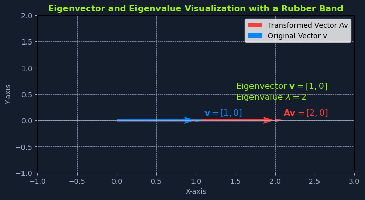
Consider a rubber band stretched along a coordinate system. A vector can represent the rubber band, and we can transform it using a matrix.
Let's say the rubber band is initially aligned with the x-axis and has a length of 1 unit. This can be represented by the vector v = [1, 0].
Now, imagine applying a linear transformation (stretching it) represented by the matrix A:
Code: python
A = [[2, 0],
     [0, 1]]
When we multiply the matrix A by the vector v, we get:
Code: python
A * v = [[2, 0],
         [0, 1]] * [1, 0] = [2, 0]
The resulting vector is [2, 0], which points in the same direction as the original vector v but has been stretched by a factor of 2. The eigenvector is v = [1, 0], and the corresponding eigenvalue is λ = 2.
In Principal Component Analysis (PCA), the eigenvalue equation helps identify the principal components of the data. The principal components are obtained by solving the following eigenvalue equation:
Code: python
C * v = λ * v
Where:
C is the standardized data's covariance matrix. This matrix represents the relationships between different features, with each element indicating the covariance between two features.v is the eigenvector. Eigenvectors represent the directions of the principal components in the feature space, indicating the directions of maximum variance in the data.λ is the eigenvalue. Eigenvalues represent the amount of variance explained by each corresponding eigenvector (principal component). Larger eigenvalues correspond to eigenvectors that capture more variance.Solving this equation involves finding the eigenvectors and eigenvalues of the covariance matrix. This can be done using techniques like:
Eigenvalue Decomposition: Directly computing the eigenvalues and eigenvectors.Singular Value Decomposition (SVD): A more numerically stable method that decomposes the data matrix into singular vectors and singular values related to the eigenvectors and eigenvalues of the covariance matrix.Once the eigenvectors and eigenvalues are found, they are sorted in descending order of their corresponding eigenvalues. The top k eigenvectors (those with the largest eigenvalues) are selected to form the new feature space. These top k eigenvectors represent the principal components that capture the most significant variance in the data.
The transformation of the original data X into the lower-dimensional representation Y can be expressed as:
Code: python
Y = X * V
Where:
Y is the transformed data matrix in the lower-dimensional space.X is the original data matrix.V is the matrix of selected eigenvectors.This transformation projects the original data points onto the new feature space defined by the principal components, resulting in a lower-dimensional representation that captures the most significant variance in the data. This reduced representation can be used for various purposes such as visualization, noise reduction, and improving the performance of machine learning models.
The number of principal components to retain is a crucial decision in PCA. It determines the trade-off between dimensionality reduction and information preservation.
A common approach is to plot the explained variance ratio against the number of components. The explained variance ratio indicates the proportion of total variance captured by each principal component. By examining the plot, you can choose the number of components that capture a sufficiently high percentage of the total variance (e.g., 95%). This ensures that the reduced representation retains most of the essential information from the original data.
PCA makes certain assumptions about the data:
Linearity: It assumes that the relationships between features are linear.Correlation: It works best when there is a significant correlation between features.Scale: It is sensitive to the scale of the features, so it is important to standardize the data before applying PCA.PCA is a powerful technique for dimensionality reduction and data analysis. It can simplify complex datasets, extract meaningful features, and visualize data in a lower-dimensional space. However, knowing its assumptions and limitations is important to ensure its effective and appropriate application.
Anomaly detection, also known as outlier detection, is crucial in unsupervised learning. It identifies data points that deviate significantly from normal behavior within a dataset. These anomalous data points, often called outliers, can indicate critical events, such as fraudulent activities, system failures, or medical emergencies.
Think of it like a security system that monitors a building. The system learns the normal activity patterns, such as people entering and exiting during business hours. It raises an alarm if it detects something unusual, like someone trying to break in at night. Similarly, anomaly detection algorithms learn the normal patterns in data and flag any deviations as potential anomalies.
Anomalies can be broadly categorized into three types:
Point Anomalies: Individual data points significantly differ from the rest—for example, a sudden spike in network traffic or an unusually high credit card transaction amount.Contextual Anomalies: Data points considered anomalous within a specific context but not necessarily in isolation. For example, a temperature reading of 30°C might be expected in summer but anomalous in winter.Collective Anomalies: A group of data points that collectively deviate from the normal behavior, even though individual data points might not be considered anomalous. For example, a sudden surge in login attempts from multiple unknown IP addresses could indicate a coordinated attack.Various techniques are employed for anomaly detection, including:
Statistical Methods: These methods assume that normal data points follow a specific statistical distribution (e.g., Gaussian distribution) and identify outliers as data points that deviate significantly from this distribution. Examples include z-score, modified z-score, and boxplots.Clustering-Based Methods: These methods group similar data points together and identify outliers as data points that do not belong to any cluster or belong to small, sparse clusters. K-means clustering and density-based clustering are commonly used for anomaly detection.Machine Learning-Based Methods: These methods utilize machine learning algorithms to learn patterns from normal data and identify outliers as data points that do not conform to these patterns. Examples include One-Class SVM, Isolation Forest, and Local Outlier Factor (LOF).
One-Class SVM is a machine learning algorithm specifically designed for anomaly detection. It learns a boundary that encloses the normal data points and identifies any data point falling outside this boundary as an outlier. It's like drawing a fence around a sheep pen – any sheep found outside the fence is likely an anomaly. One-Class SVM can handle non-linear relationships using kernel functions, similar to SVMs used for classification.
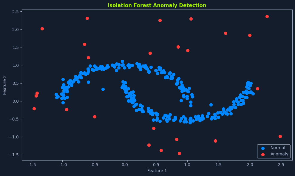
Isolation Forest is another popular anomaly detection algorithm that isolates anomalies by randomly partitioning the data and constructing isolation trees. Anomalies, being "few and different," are easier to isolate from the rest of the data and tend to have shorter paths in these trees. It's like playing a game of "20 questions" – if you can identify an object with very few questions, it's likely an anomaly.
The algorithm works by recursively partitioning the data until each data point is isolated in its leaf node. A random feature is selected at each step, and a random split value is chosen. This process is repeated until all data points are isolated.
The anomaly score for a data point is then calculated based on the average path length to isolate that data point in multiple isolation trees. Shorter path lengths indicate a higher likelihood of being an anomaly.
The anomaly score for a data point x is calculated as:
Code: python
score(x) = 2^(-E(h(x)) / c(n))
Where:
E(h(x)): Average path length of data point x in a collection of isolation trees.c(n): Average path length of unsuccessful search in a Binary Search Tree (BST) with n nodes. This serves as a normalization factor.n: Number of data points.Anomaly scores closer to 1 indicate a higher likelihood of being an anomaly, while scores closer to 0.5 indicate that the data point is likely normal.
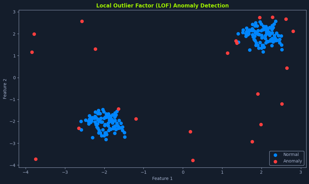
Local Outlier Factor (LOF) is a density-based algorithm designed to identify outliers in datasets by comparing the local density of a data point to that of its neighbors. It is particularly effective in detecting anomalies in regions where the density of points varies significantly.
Think of it like identifying a house in a sparsely populated area compared to a densely populated neighborhood. The isolated house in a region with fewer houses is more likely to be an anomaly. Similarly, in data terms, a point with a lower local density than its neighbors is considered an outlier.
The LOF score for a data point p is calculated using the following formula:
Code: python
LOF(p) = (Σ lrd(o) / k) / lrd(p)
Where:
lrd(p) : The local reachability density of data point p.lrd(o) : The local reachability density of data point o, one of the k nearest neighbors of p.k : The number of nearest neighbors.Higher LOF scores indicate a higher likelihood of a data point being an outlier.
The local reachability density (lrd(p)) for a data point p is defined as:
Code: python
lrd(p) = 1 / (Σ reach_dist(p, o) / k)
Where:
reach_dist(p, o): The reachability distance from p to o, which is the maximum of the actual distance between p and o and the k-distance of o.The k-distance of a point o is the distance to its kth nearest neighbor. This ensures that points in dense regions have lower reachability distances, while points in sparse regions have higher reachability distances.
Anomaly detection techniques often make certain assumptions about the data:
Normal Data Distribution: Some methods assume that normal data points, such as Gaussian distribution, follow a specific distribution.Feature Relevance: The choice of features can significantly impact the performance of anomaly detection algorithms.Labeled Data (for some methods): Some machine learning-based methods require labeled data to train the model.Anomaly detection is a critical task in data analysis and machine learning, enabling the identification of unusual patterns and events that can have significant implications. By leveraging various techniques and algorithms, anomaly detection systems can effectively identify outliers and provide valuable insights for decision-making and proactive intervention.
Reinforcement learning (RL) introduces a unique paradigm in machine learning where an agent learns by interacting with an environment. Unlike supervised learning, which relies on labeled data, or unsupervised learning, which explores unlabeled data, RL focuses on learning through trial and error, guided by feedback in the form of rewards or penalties. This approach mimics how humans learn through experience, making RL particularly suitable for tasks that involve sequential decision-making in dynamic environments.
Think of it like training a dog. You don't give the dog explicit instructions on sitting, staying, or fetching. Instead, you reward it with treats and praise when it performs the desired actions and correct it when it doesn't. The dog learns to associate specific actions with positive outcomes through trial, error, and feedback.
In RL, an agent interacts with an environment by acting and observing the consequences. The environment provides feedback through rewards or penalties, guiding the agent toward learning an optimal policy. A policy is a strategy for selecting actions that maximize cumulative rewards over time.
Reinforcement learning algorithms can be broadly categorized into:
Model-Based RL: The agent learns a model of the environment, which it uses to predict future states and plan its actions. This approach is analogous to having a map of a maze before navigating it. The agent can use this map to plan the most efficient path to the goal, reducing the need for trial and error.Model-Free RL: The agent learns directly from experience without explicitly modeling the environment. This is like navigating a maze without a map, where the agent relies solely on trial and error and feedback from the environment to learn the best actions. The agent gradually improves its policy by exploring different paths and learning from the rewards or penalties it receives.Understanding Reinforcement Learning (RL) requires a grasp of its core concepts. These concepts provide the foundation for understanding how agents learn and interact with their environment to achieve their goals.
The agent is the learner and decision-maker in an RL system. It interacts with the environment, taking action and observing the consequences. The agent aims to learn an optimal policy that maximizes cumulative rewards over time.
Think of the agent as a robot navigating a maze, a program playing a game, or a self-driving car navigating through traffic. In each case, the agent makes decisions and learns from its experiences.
The environment is the external system or context in which the agent operates. It encompasses everything outside the agent, including the physical world, a simulated world, or even a game board. The environment responds to the agent's actions and provides feedback through rewards or penalties.
In the maze navigation example, the environment is the maze itself, with its walls, paths, and goal location. In a game-play scenario, the environment is the game with its rules and opponent moves.
The state represents the current situation or condition of the environment. It provides a snapshot of the relevant information that the agent needs to make informed decisions. The state can include various aspects of the environment, such as the agent's position, the positions of other objects, and any other relevant variables.
The state of a robot navigating a maze might include its current location and the surrounding walls. In a chess game, the state is the current configuration of the chessboard.
An action is an agent's move or decision that affects the environment. The agent selects actions based on its current state and its policy. The environment responds to the action and transitions to a new state.
In the maze example, the robot's actions might be to move forward, turn left, or turn right. In a game, the actions might be to move a piece or make a specific play.
The reward is feedback from the environment indicating the desirability of the agent's action. It is a scalar value that can be positive, negative, or zero. Positive rewards encourage the agent to repeat the action, while negative rewards (penalties) discourage it. The agent's goal is to maximize cumulative rewards over time.
In the maze example, the robot might receive a positive reward for getting closer to the goal and a penalty for hitting a wall. In a game, the reward might be positive for winning and negative for losing.
A policy is a strategy or mapping from states to actions the agent follows. It determines which action the agent should take in a given state. The agent aims to learn an optimal policy that maximizes cumulative rewards.
The policy can be deterministic, where it always selects the same action in a given state, or stochastic, where it selects actions with certain probabilities.
The value function estimates the long-term value of being in a particular state or taking a specific action. It predicts the expected cumulative reward that the agent can obtain from that state or action onwards. The value function is a crucial component in many RL algorithms, as it guides the agent towards choosing actions that lead to higher long-term rewards.
There are two main types of value functions:
State-value function: Estimates the expected cumulative reward from starting in a given state and following a particular policy.Action-value function: Estimates the expected cumulative reward from taking a specific action in a given state and then following a particular policy.The discount factor (γ) is a RL parameter that determines future rewards' present value. It ranges between 0 and 1, with values closer to 1 giving more weight to long-term rewards and values closer to 0 emphasizing short-term rewards.
γ=0 means the agent only considers immediate rewards.γ=1 means the agent values all future rewards equally.Episodic tasks involve the agent interacting with the environment in episodes, each ending at a terminal state (e.g., reaching the goal in a maze). In contrast, continuous tasks have no explicit end and continue indefinitely (e.g., controlling a robot arm).
Q-learning is a model-free reinforcement learning algorithm that learns an optimal policy by estimating the Q-value. The Q-value represents the expected cumulative reward an agent can obtain by taking a specific action in a given state and following the optimal policy afterward. It's called "model-free" because the agent doesn't need a prior model of the environment to learn; it learns directly through trial and error, interacting with the environment and observing the outcomes.
Imagine a self-driving car learning to navigate a city. It starts without knowing the roads, traffic lights, or pedestrian crossings. Through Q-learning, the car explores the city, taking actions (accelerating, braking, turning) and receiving rewards (for reaching destinations quickly and safely) or penalties (for collisions or traffic violations). Over time, the car learns which actions lead to higher rewards in different situations, eventually mastering the art of driving in that city.
At the heart of Q-learning lies the Q-table. This table is a core algorithm component, storing the Q-values for all possible state-action pairs. Think of it as a lookup table that guides the agent's decision-making process. The rows of the table represent the states (e.g., different locations in the city for the self-driving car), and the columns represent the actions (e.g., accelerate, brake, turn left, turn right). Each cell in the table holds the Q-value for taking a particular action in a particular state.
Below is an illustration of a simple Q-table for a grid world environment where a robot can move up, down, left, or right. The grid cells represent the states, and the actions are the possible movements.
| State/Action | Up | Down | Left | Right |
|---|---|---|---|---|
| S1 | -1.0 | 0.0 | -0.5 | 0.2 |
| S2 | 0.0 | 1.0 | 0.0 | -0.3 |
| S3 | 0.5 | -0.5 | 1.0 | 0.0 |
| S4 | -0.2 | 0.0 | -0.3 | 1.0 |
In this table, S1, S2, S3, and S4 are different states in the grid world. The values in the cells represent the Q-values for taking each action from each state.
The Q-value for a particular state-action pair is updated using the Q-learning update rule, which is based on the Bellman equation:
Q(s, a) = Q(s, a) + α * [r + γ * max(Q(s', a')) - Q(s, a)]
Where:
Q(s, a) is the current Q-value for taking action a in state s.α (alpha) is the learning rate, which determines the weight given to new information.r is the reward received after taking action a from state s.γ (gamma) is the discount factor, which determines the importance of future rewards.max(Q(s', a')) is the maximum Q-value of the next state s' and any action a'.Let's use an example of updating a Q-value for the robot in the grid world environment.
S1.Right, moving to state S2.r = 0.5 for reaching state S2.α = 0.1.γ = 0.9.Q-value of the next state S2 is max(Q(S2, Up), Q(S2, Down), Q(S2, Left), Q(S2, Right)) = max(0.0, 1.0, 0.0, -0.3) = 1.0.Using the Q-learning update rule:
Q(S1, Right) = Q(S1, Right) + α * [r + γ * max(Q(S2, a')) - Q(S1, Right)]
Q(S1, Right) = 0.2 + 0.1 * [0.5 + 0.9 * 1.0 - 0.2]
Q(S1, Right) = 0.2 + 0.1 * [0.5 + 0.9 - 0.2]
Q(S1, Right) = 0.2 + 0.1 * 1.2
Q(S1, Right) = 0.2 + 0.12
Q(S1, Right) = 0.32
After updating, the new Q-value for taking action Right from state S1 is 0.32. This updated value reflects the robot's learning from the experience of moving to state S2 and receiving a reward.

The Q-learning algorithm is an iterative process of action selection, observation, and Q-value updates. The agent continuously interacts with the environment, learning from its experiences and refining its policy to maximize cumulative rewards.
Here's a breakdown of the steps involved:
Initialization: The Q-table is initialized, typically with arbitrary values (e.g., all zeros) or with some prior knowledge if available. This table will be updated as the agent learns.Choose an Action: In the current state, the agent selects an action to execute. This selection involves balancing exploration (trying new actions to discover potentially better strategies) and exploitation (using the current best-known action to maximize reward). This balance ensures that the agent explores the environment sufficiently while capitalizing on existing knowledge.Take Action and Observe: The agent performs the chosen action in the environment and observes the consequences. This includes the new state it transitions to after taking the action and the immediate reward received from the environment. These observations provide valuable feedback to the agent about the effectiveness of its actions.Update Q-value: The Q-value for the state-action pair is updated using the Q-learning update rule, which incorporates the received and estimated future rewards from the new state.Update State: The agent updates its current state to the new state it transitioned to after taking the action. This sets the stage for the next iteration of the algorithm.Iteration: Steps 2-5 are repeated until the Q-values converge to their optimal values, indicating that the agent has learned an effective policy, or a predefined stopping condition is met (e.g., a maximum number of iterations or a time limit).This iterative process allows the agent to continuously learn and refine its policy, improving its decision-making abilities and maximizing its cumulative rewards over time.
Ultimately, the agent successfully navigates from the start to the goal by following the path that maximizes the cumulative reward.
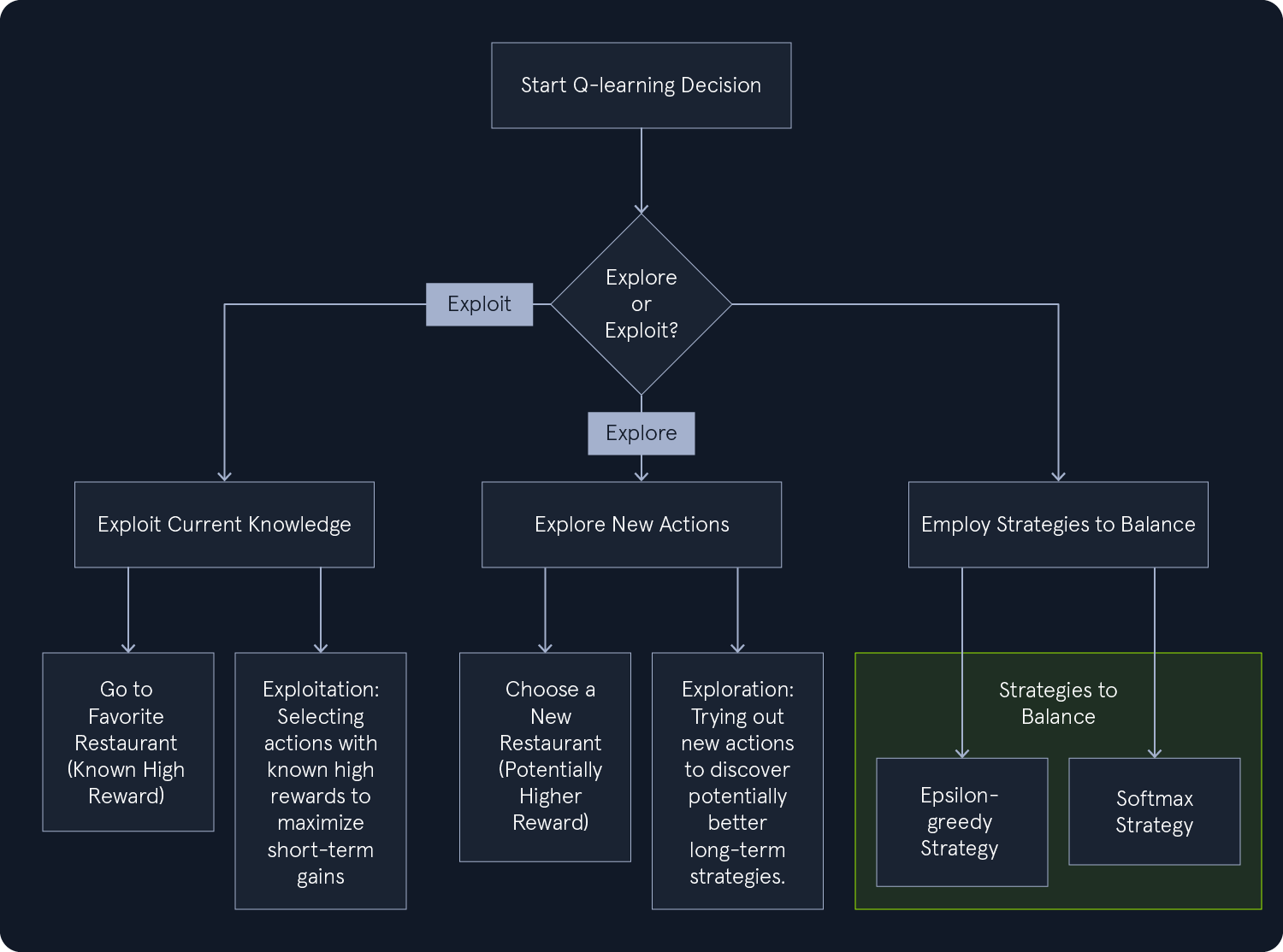
In Q-learning, the agent faces a fundamental dilemma: Should it explore new actions to discover better strategies potentially, or should it exploit its current knowledge and choose actions that have yielded high rewards in the past? This is the exploration-exploitation trade-off, a crucial aspect of reinforcement learning.
Think of it like choosing a restaurant for dinner. You could exploit your existing knowledge and go to your favorite restaurant, where you know you'll enjoy the food. Or, you could explore a new restaurant, taking a chance to discover a hidden gem you might like even more.
Q-learning employs various strategies to balance exploration and exploitation. The goal is to find a balance that allows the agent to learn effectively while maximizing its rewards.
Exploration: Encourages the agent to try different actions, even if they haven't previously led to high rewards. This helps the agent discover new and potentially better strategies.Exploitation: This strategy focuses on selecting actions that have previously resulted in high rewards. It allows the agent to capitalize on existing knowledge and maximize short-term gains.The epsilon-greedy strategy offers a simple yet effective approach to balancing exploration and exploitation in Q-learning. It introduces randomness into the agent's action selection, preventing it from always defaulting to the same actions and potentially missing out on more rewarding options.
The epsilon-greedy strategy encourages you to explore new options while still allowing you to enjoy your known favorites. With probability epsilon (ε), you venture out and try a random coffee shop, potentially discovering a hidden gem. With probability 1-epsilon, you stick to your usual spot, ensuring a satisfying coffee experience.
The value of epsilon is a key parameter that can be adjusted over time to fine-tune the balance between exploration and exploitation.
High Epsilon (e.g., 0.9): A high epsilon value initially promotes more exploration. This is like being new in town and eager to try different coffee shops to find the best one.Low Epsilon (e.g., 0.1): As you gain more experience and develop preferences, you might decrease epsilon. This is like becoming a regular at your favorite coffee shop while occasionally trying new places.Q-learning makes minimal assumptions about the data:
Markov Property: It assumes that the environment satisfies the Markov property, meaning that the next state depends only on the current state and action, not on the history of previous states and actions.Stationary Environment: It assumes that the environment's dynamics (transition probabilities and reward functions) do not change over time.Q-learning is a powerful and versatile algorithm for learning optimal policies in reinforcement learning problems. Its ability to learn without a model of the environment makes it suitable for a wide range of applications where the environment's dynamics are unknown or complex.

SARSA is a model-free reinforcement learning algorithm that learns an optimal policy through direct environmental interaction. Unlike Q-learning, which updates its Q-values based on the maximum Q-value of the next state, SARSA updates its Q-values based on the Q-value of the next state and the actual action taken in that state. This key difference makes SARSA an on-policy algorithm, meaning it learns the value of the policy it is currently following. Q-learning is off-policy, learning the value of the optimal policy independent of the current policy.
The update rule for SARSA is:
Code: python
Q(s, a) <- Q(s, a) + α * (r + γ * Q(s', a') - Q(s, a))
Here, s is the current state, a is the current action, r is the reward received, s' is the next state, a' is the next action taken, α is the learning rate, and γ is the discount factor. The term Q(s', a') reflects the expected future reward for the next state-action pair, which the current policy determines.
This conservative approach makes SARSA suitable for environments where policy needs to be followed closely. At the same time, Q-Learning's more exploratory nature can more efficiently find optimal policies in some cases.
Imagine a robot learning to navigate a room with obstacles. SARSA guides the robot to learn a safe path by considering the immediate reward of an action and the consequences of the next action taken in the new state. This cautious approach helps the robot avoid risky actions that might lead to collisions, even if those actions initially seem promising.
The SARSA algorithm follows these steps:
Initialization: Initialize the Q-table with arbitrary values (usually 0) for each state-action pair. This table will store the estimated Q-values for actions in different states.Choose an Action: In the current state s, select an action a to execute. This selection is typically based on an exploration-exploitation strategy, such as epsilon-greedy, balancing exploring new actions with exploiting actions known to yield high rewards.Take Action and Observe: Execute the chosen action a in the environment and observe the next state s' and the reward r received. This step involves interacting with the environment and gathering feedback on the consequences of the action.Choose Next Action: In the next state s', select the next action a' based on the current policy (e.g., epsilon-greedy). This step is crucial for SARSA's on-policy nature, considering the actual action taken in the next state, not just the theoretically optimal action.Update Q-value: Update the Q-value for the state-action pair (s, a).Update State and Action: Update the current state and action to the next state and action: s = s', a = a'. This prepares the algorithm for the next iteration.Iteration: Repeat steps 2-6 until the Q-values converge or a maximum number of iterations is reached. This iterative process allows the agent to learn and refine its policy continuously._0.png)
In reinforcement learning, the learning process can be categorized into two main approaches: on-policy and off-policy learning. This distinction stems from how algorithms update their estimates of action values, which are crucial for determining the optimal policy.
On-policy learning: In on-policy learning, the algorithm learns the value of its current policy. This means that the updates to the estimated action values are based on the actions taken and the rewards received while executing the current policy, including any exploratory actions.Off-policy learning: In contrast, off-policy learning allows the algorithm to learn about an optimal policy independently of the policy being followed for action selection. This means the algorithm can learn from data generated by a different policy, which can benefit exploration and learning from historical data._1.png)
SARSA's on-policy nature stems from its unique update rule. It uses the Q-value of the next state and the actual action taken in that next state, according to the current policy, to update the Q-value of the current state-action pair. This contrasts with Q-learning, which uses the maximum Q-value over all possible actions in the next state, regardless of the current policy.
This distinction has important implications:
Learning the Value of the Current Policy: SARSA learns the value of its current policy, including the exploration steps. This means it estimates the expected return for taking actions according to the current policy, which might involve some exploratory moves.Safety and Stability: On-policy learning can be advantageous in situations where safety and stability are critical. Since SARSA learns by following the current policy, it is less likely to explore potentially dangerous or unstable actions that could lead to negative consequences.Exploration Influence: The exploration strategy (e.g., epsilon-greedy) influences learning. SARSA learns the policy's value, including exploration, so the learned Q-values reflect the balance between exploration and exploitation.In essence, SARSA learns "on the job," continuously updating its estimates based on the actions taken and the rewards received while following its current policy. This makes it suitable for scenarios where learning a safe and stable policy is a priority, even if it means potentially sacrificing some optimality.
Just like Q-learning, SARSA also faces the exploration-exploitation dilemma. The agent must balance exploring new actions to discover potentially better strategies and exploiting its current knowledge to maximize rewards. The choice of exploration-exploitation strategy influences the learning process and the resulting policy.
_2.png)
As discussed in Q-learning, the epsilon-greedy strategy involves selecting a random action with probability epsilon (ε) and the greedy action (highest Q-value) with probability 1-ε. This approach balances exploration and exploitation by occasionally choosing random actions to discover potentially better options.
In SARSA, the epsilon-greedy strategy leads to more cautious exploration. The agent considers the potential consequences of exploratory actions in the next state, ensuring that they do not deviate too far from known good policies.
_3.png)
The softmax strategy assigns probabilities to actions based on their Q-values, with higher Q-values leading to higher probabilities. This allows for a smoother exploration, where actions with moderately high Q-values still can be selected, promoting a more balanced approach to exploration and exploitation.
In SARSA, the softmax strategy can lead to more nuanced and adaptive behavior. It encourages the agent to explore actions that are not necessarily the best but are still promising, thereby potentially leading to better long-term outcomes.
The choice of exploration-exploitation strategy in SARSA depends on the specific problem and the desired balance between safety and optimality. A more exploratory strategy might lead to a longer learning process but potentially a more optimal policy. A more conservative strategy might lead to faster learning but potentially a suboptimal policy that avoids risky actions.
Like other iterative algorithms, SARSA requires careful parameter tuning to ensure convergence to an optimal policy. Convergence in Reinforcement Learning means the algorithm reaches a stable solution where the Q-values no longer change significantly with further training. This indicates that the agent has learned a policy that effectively maximizes rewards.
Two crucial parameters that influence the learning process are the learning rate (α) and the discount factor (γ):
Learning Rate (α): Controls the extent of Q-value updates in each iteration. A high α leads to faster updates but can cause instability, while a low α ensures more stable convergence but slows down learning.Discount Factor (γ): Determines the importance of future rewards relative to immediate rewards. A high γ (close to 1) emphasizes long-term rewards, while a low γ prioritizes immediate rewards.Tuning these parameters often involves experimentation to find a balance that ensures stable and efficient learning. Techniques like grid search or cross-validation can systematically explore different parameter combinations to identify optimal settings for a given problem.
The convergence of SARSA also depends on the exploration-exploitation strategy and the nature of the environment. SARSA is guaranteed to converge to an optimal policy under certain conditions, such as when the learning rate is sufficiently small, and the exploration strategy ensures that all state-action pairs are visited infinitely often.
SARSA makes similar assumptions to Q-learning:
Markov Property: It assumes that the environment satisfies the Markov property, meaning that the next state depends only on the current state and action, not on the history of previous states and actions.Stationary Environment: It assumes that the environment's dynamics (transition probabilities and reward functions) do not change over time.SARSA is a valuable reinforcement learning algorithm that offers an on-policy learning approach, making it suitable for scenarios where safety and stability are critical considerations. Its ability to learn by following a specific policy allows it to find effective solutions while avoiding potentially harmful actions.
Deep learning is a subfield of machine learning that has emerged as a powerful force in artificial intelligence. It uses artificial neural networks with multiple layers (hence "deep") to analyze data and learn complex patterns. These networks are inspired by the structure and function of the human brain, enabling them to achieve remarkable performance on various tasks.
Deep learning can be viewed as a specialized subset of machine learning. While traditional machine learning algorithms often require manual feature engineering, deep learning algorithms can automatically learn relevant features from raw data. This ability to learn hierarchical representations of data sets deep learning apart and enables it to tackle more complex problems.
In the broader context of AI, deep learning plays a crucial role in achieving the goals of creating intelligent agents and solving complex problems. Deep learning models are now used in various AI applications, including natural language processing, computer vision, robotics, and more.
The motivation behind deep learning stems from two primary goals:
Solving Complex Problems: Deep learning has proven highly effective in solving complex problems that previously challenged traditional AI approaches. Its ability to learn intricate patterns from vast amounts of data has led to breakthroughs in image recognition, speech processing, and natural language understanding.Mimicking the Human Brain: The architecture of deep neural networks is inspired by the interconnected network of neurons in the human brain. This allows deep learning models to process information hierarchically, similar to how humans perceive and understand the world. Deep learning aims to create AI systems that can learn and reason more effectively by mimicking the human brain.Deep learning has emerged as a transformative technology that can revolutionize various fields. Its ability to solve complex problems and mimic the human brain makes it a key driver of progress in artificial intelligence.
To understand deep learning, it's essential to grasp some key concepts that underpin its structure and functionality.
Artificial Neural Networks (ANNs) are computing systems inspired by the biological neural networks that constitute animal brains. An ANN is composed of interconnected nodes or neurons organized in layers. Each connection between neurons has a weight associated with it, representing the strength of the connection.
The network learns by adjusting these weights based on the input data, enabling it to make predictions or decisions. ANNs are fundamental to deep learning, as they provide the framework for building complex models that can learn from vast amounts of data.
Deep learning networks are characterized by their layered structure. There are three main types of layers:
Input Layer: This layer receives the initial data input.Hidden Layers: These intermediate layers perform computations and extract features from the data. Deep learning networks have multiple hidden layers, allowing them to learn complex patterns.Output Layer: This layer produces the network's final output, such as a prediction or classification.Activation functions introduce non-linearity into the network, enabling it to learn complex patterns. They determine whether a neuron should be activated based on its input. Common activation functions include:
Sigmoid: Squashes the input into a range between 0 and 1.ReLU (Rectified Linear Unit): Returns 0 for negative inputs and the input value for positive inputs.Tanh (Hyperbolic Tangent): Squashes the input into a range between -1 and 1.Backpropagation is a key algorithm used to train deep learning networks. It involves calculating the gradient of the loss function concerning the network's weights and then updating the weights in the direction that minimizes the loss. This iterative process allows the network to learn from the data and improve its performance over time.
The loss function measures the error between the network's predictions and the actual target values. The goal of training is to minimize this loss function. Different tasks require different loss functions. For example, mean squared error is commonly used for regression tasks, while cross-entropy loss is used for classification tasks.
The optimizer determines how the network's weights are updated during training. It uses the gradients calculated by backpropagation to adjust the weights to minimize the loss function. Popular optimizers include:
Stochastic Gradient Descent (SGD)AdamRMSpropHyperparameters are set before training begins and control the learning process. Examples include the learning rate, the number of hidden layers, and the number of neurons in each layer. Tuning hyperparameters is crucial for achieving optimal performance.
These concepts form the building blocks of deep learning. Understanding them is crucial for comprehending how deep learning models are constructed, trained, and used to solve complex problems.
The perceptron is a fundamental building block of neural networks. It is a simplified model of a biological neuron that can make basic decisions. Understanding perceptrons is crucial for grasping the concepts behind more complex neural networks used in deep learning.
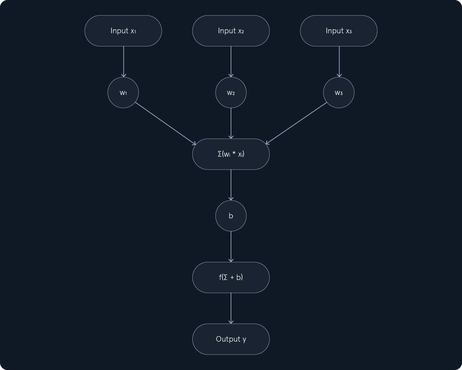
A perceptron consists of the following components:
Input Values (x1, x2, ..., xn): These are the initial data points fed into the perceptron. Each input value represents a feature or attribute of the data.Weights (w1, w2, ..., wn): Each input value is associated with a weight, determining its strength or importance. Weights can be positive or negative and influence the output of the perceptron.Summation Function (∑): The weighted inputs are summed together as ∑(wi * xi) . This step aggregates the weighted inputs into a single value.Bias (b): A bias term is added to the weighted sum to shift the activation function. It allows the perceptron to activate even when all inputs are zero.Activation Function (f): The activation function introduces non-linearity into the perceptron. It takes the weighted sum plus the bias as input and produces an output based on a predefined threshold.Output (y): The final output of the perceptron, typically a binary value (0 or 1) representing a decision or classification.In essence, a perceptron takes a set of inputs, multiplies them by their corresponding weights, sums them up, adds a bias, and then applies an activation function to produce an output. This simple yet powerful structure forms the basis of more complex neural networks used in deep learning.
Let's illustrate the functionality of a perceptron with a simple example: deciding whether to play tennis based on weather conditions. We'll consider four input features:
Outlook: Sunny (0), Overcast (1), Rainy (2)Temperature: Hot (0), Mild (1), Cool (2)Humidity: High (0), Normal (1)Wind: Weak (0), Strong (1)Our perceptron will take these inputs and output a binary decision: Play Tennis (1) or Don't Play Tennis (0).
For simplicity, let's assume the following weights and bias:
w1 (Outlook) = 0.3w2 (Temperature) = 0.2w3 (Humidity) = -0.4w4 (Wind) = -0.2b (Bias) = 0.1We'll use a simple step activation function:
f(x) = 1 if x > 0, else 0
Implemented in Python, like this:
def step_activation(x):
  """Step activation function."""
  return 1 if x > 0 else 0
Now, let's consider a day with the following conditions:
Outlook: Sunny (0)Temperature: Mild (1)Humidity: High (0)Wind: Weak (0)The perceptron calculates the weighted sum:
(0.3 * 0) + (0.2 * 1) + (-0.4 * 0) + (-0.2 * 0) = 0.2
Adding the bias:
Code: python
0.2 + 0.1 = 0.3
Applying the activation function:
f(0.3) = 1 (since 0.3 > 0)
The output is 1, so the perceptron decides to Play Tennis.
In Python, this looks like this:
# Input features
outlook = 0
temperature = 1
humidity = 0
wind = 0

# Weights and bias
w1 = 0.3
w2 = 0.2
w3 = -0.4
w4 = -0.2
b = 0.1

# Calculate weighted sum
weighted_sum = (w1 * outlook) + (w2 * temperature) + (w3 * humidity) + (w4 * wind)

# Add bias
total_input = weighted_sum + b

# Apply activation function
output = step_activation(total_input)

print(f"Output: {output}")  # Output: 1 (Play Tennis)
This basic example demonstrates how a perceptron can weigh different inputs and make a binary decision based on a simple activation function. In real-world scenarios, perceptrons are often combined into complex networks to solve more intricate tasks.
While perceptrons provide a foundational understanding of neural networks, single-layer perceptrons have significant limitations that restrict their applicability to more complex tasks.
The most notable limitation is their inability to solve problems that are not linearly separable. A dataset is considered linearly separable if it can be divided into two classes by a single straight line (or hyperplane in higher dimensions). Single-layer perceptrons can only learn linear decision boundaries, making them incapable of classifying data with non-linear patterns.
A classic example is the XOR problem. The XOR function returns true (1) if only one of the inputs is true and false (0) otherwise. It's impossible to draw a single straight line that separates the true and false outputs of the XOR function. This limitation severely restricts the types of problems a single-layer perceptron can solve.
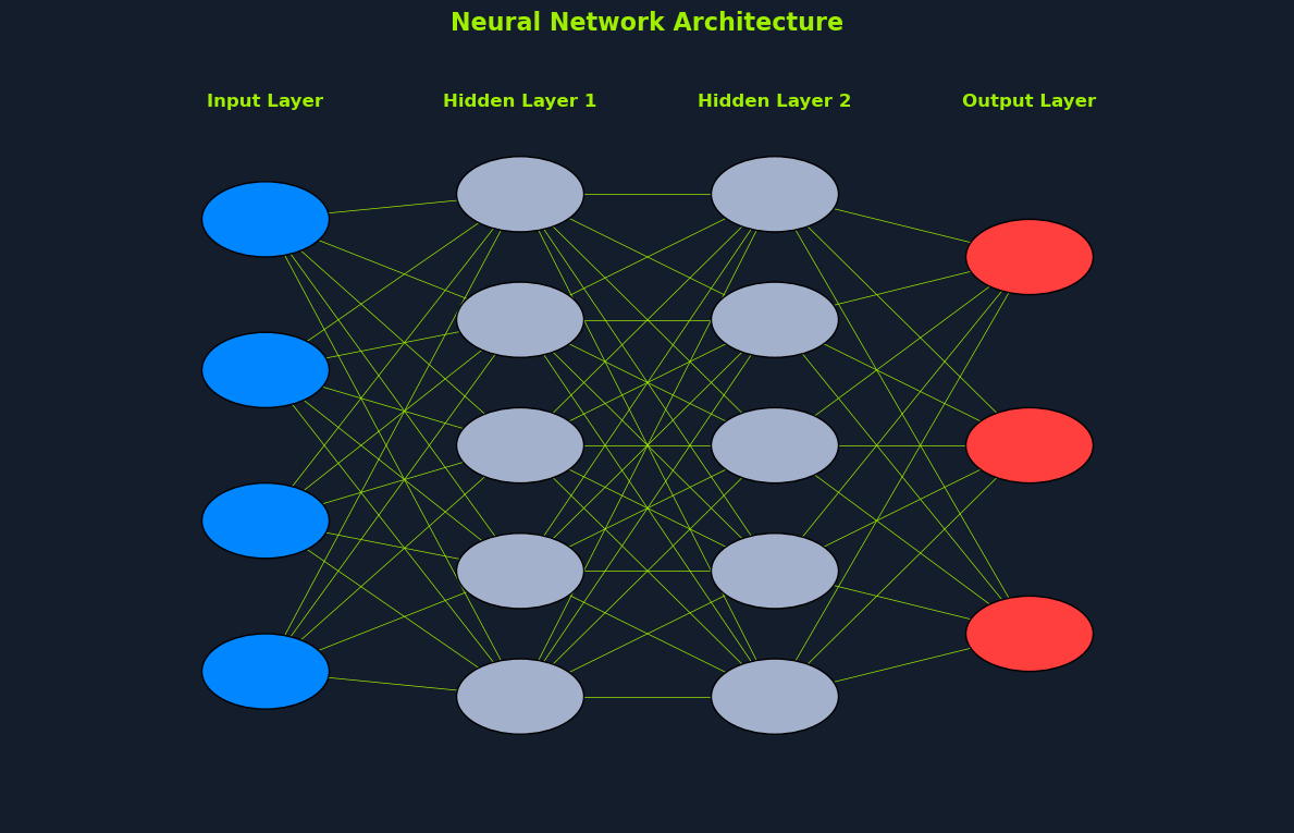
To overcome the limitations of single-layer perceptrons, we introduce the concept of neural networks with multiple layers. These networks, also known as multi-layer perceptrons (MLPs), are composed of:
A neuron is a fundamental computational unit in neural networks. It receives inputs, processes them using weights and a bias, and applies an activation function to produce an output. Unlike the perceptron, which uses a step function for binary classification, neurons can use various activation functions such as the sigmoid, ReLU, and tanh.
This flexibility allows neurons to handle non-linear relationships and produce continuous outputs, making them suitable for various tasks.
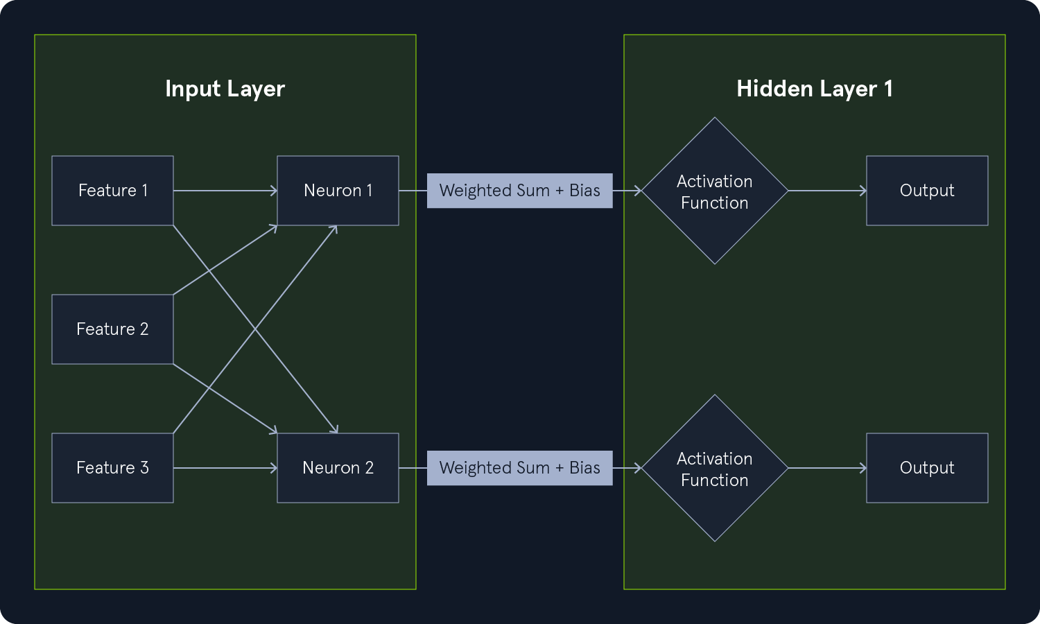
The input layer serves as the entry point for the data. Each neuron in the input layer corresponds to a feature or attribute of the input data. The input layer passes the data to the first hidden layer.
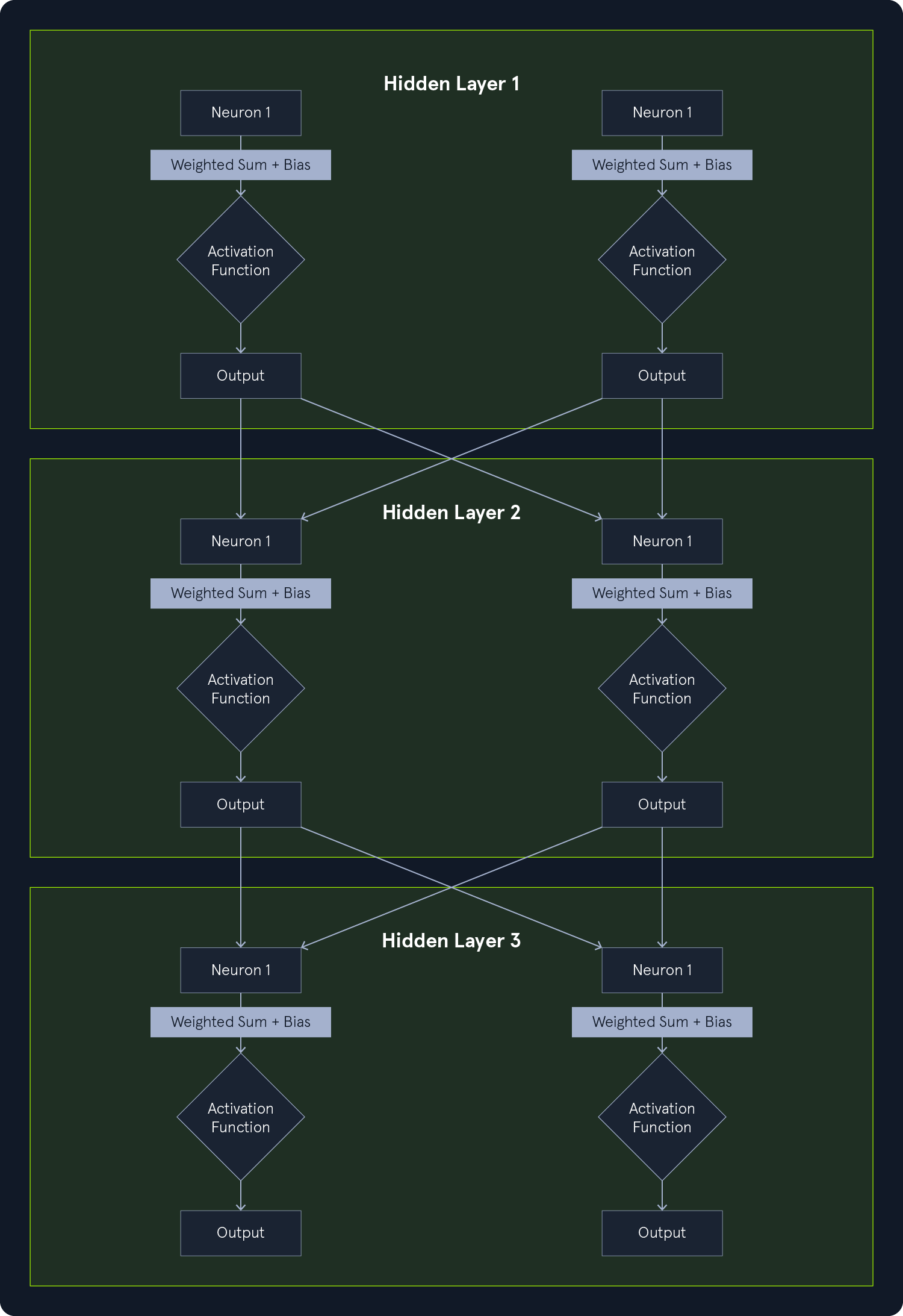
Hidden layers are the intermediate layers between the input and output layers. They perform computations and extract features from the data. Each neuron in a hidden layer:
The output of each neuron in a hidden layer is then passed as input to the next layer.
Multiple hidden layers allow the network to learn complex non-linear relationships within the data. Each layer can learn different levels of abstraction, with the initial layers learning simple features and subsequent layers combining those features into more complex representations.

The output layer produces the network's final result. The number of neurons in the output layer depends on the specific task:
Multi-layer perceptrons (MLPs) overcome the limitations of single-layer perceptrons primarily by learning non-linear decision boundaries. By incorporating multiple hidden layers with non-linear activation functions, MLPs can approximate complex functions and capture intricate patterns in data that are not linearly separable.
This enables them to solve problems like the XOR problem, which single-layer perceptrons cannot address. Additionally, the hierarchical structure of MLPs allows them to learn increasingly complex features at each layer, leading to greater expressiveness and improved performance in a broader range of tasks.
Activation functions play a crucial role in neural networks by introducing non-linearity. They determine a neuron's output based on its input. Without activation functions, the network would essentially be a linear model, limiting its ability to learn complex patterns.
Each neuron in a hidden layer receives a weighted sum of inputs from the previous layer plus a bias term. This sum is then passed through an activation function, determining whether the neuron should be "activated" and to what extent. The output of the activation function is then passed as input to the next layer.
There are various activation functions, each with its own characteristics and applications. Some common ones include:
Sigmoid: The sigmoid function squashes the input into a range between 0 and 1. It was historically popular but is now less commonly used due to issues like vanishing gradients.ReLU (Rectified Linear Unit): ReLU is a simple and widely used activation function. It returns 0 for negative inputs and the input value for positive inputs. ReLU often leads to faster training and better performance.Tanh (Hyperbolic Tangent): The tanh function squashes the input into a range between -1 and 1. It is similar to the sigmoid function but centered at 0.Softmax: The softmax function is often used in the output layer for multi-class classification problems. It converts a vector of raw scores into a probability distribution over the classes.The choice of activation function depends on the specific task and network architecture.
Training a multi-layer perceptron (MLP) involves adjusting the network's weights and biases to minimize the error between its predictions and target values. This process is achieved through a combination of backpropagation and gradient descent.

Backpropagation is an algorithm for calculating the gradient of the loss function concerning the network's weights and biases. It works by propagating the error signal back through the network, layer by layer, starting from the output layer.
Here's a simplified overview of the backpropagation process:
Forward Pass: The input data is fed through the network, and the output is calculated.Calculate Error: A loss function calculates the difference between the predicted output and the actual target value.Backward Pass: The error signal is propagated back through the network. For each layer, the gradient of the loss function concerning the weights and biases is calculated using the calculus chain rule.Update Weights and Biases: The weights and biases are updated to reduce errors. This is typically done using an optimization algorithm like gradient descent.
Gradient descent is an iterative optimization algorithm used to find the minimum of a function. In the context of MLPs, the loss function is minimized.
Gradient descent works by taking steps toward the negative gradient of the loss function. The size of the step is determined by the learning rate, a hyperparameter that controls how quickly the network learns.
Here's a simplified explanation of gradient descent:
Initialize Weights and Biases: Start with random values for the weights and biases.Calculate Gradient: Use backpropagation to calculate the gradient of the loss function with respect to the weights and biases.Update Weights and Biases: Subtract a fraction of the gradient from the current weights and biases. The learning rate determines the fraction.Repeat: Repeat steps 2 and 3 until the loss function converges to a minimum or a predefined number of iterations is reached.Backpropagation and gradient descent work together to train MLPs. Backpropagation calculates the gradients, while gradient descent uses those gradients to update the network's parameters and minimize the loss function. This iterative process allows the network to learn from the data and improve its performance over time.
Convolutional Neural Networks (CNNs) are specialized neural networks designed for processing grid-like data, such as images. They excel at capturing spatial hierarchies of features, making them highly effective for tasks like image recognition, object detection, and image segmentation.
A typical CNN consists of three main types of layers:
Convolutional Layers: These are the core building blocks of a CNN. They perform convolutions on the input data using a set of learnable filters. Each filter slides across the input, computing the dot product between the filter weights and the input values at each position. This process extracts features from the input, such as edges, corners, and textures. The output of a convolutional layer is a feature map, which highlights the presence of the learned features in the input. Multiple filters are used in each layer to detect different types of features.Pooling Layers: These layers reduce the dimensionality of the feature maps, making the network less computationally expensive and less susceptible to overfitting. They operate on each feature map independently, downsampling it by taking the maximum or average value within a small window. Common types of pooling include max pooling and average pooling.Fully Connected Layers: These layers are similar to those in MLPs. They connect every neuron in one layer to every neuron in the next layer. These layers are typically used towards the network's end to perform high-level reasoning and make predictions based on the extracted features.Convolutional and pooling layers are stacked alternately to create a hierarchy of features. The output of the final pooling layer is then flattened and fed into one or more fully connected layers for classification or regression.
This layered structure lets CNNs learn complex patterns and representations from image data. The convolutional layers extract local features, the pooling layers downsample and aggregate these features, and the fully connected layers combine the high-level features to make predictions.
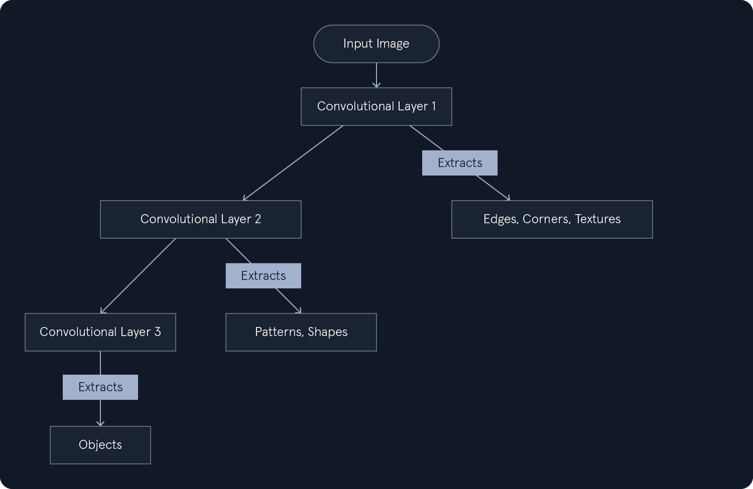
In a CNN, feature maps are generated by the convolutional layers. Each convolutional filter produces a corresponding feature map, highlighting the locations and strength of specific visual patterns within the input image. For example, one filter might detect edges, another corners, and another texture.
The network learns these features by adjusting filter weights during training. As it is exposed to more data, it refines these filters to become detectors for increasingly complex visual elements.
This learning process is hierarchical:
Initial Layers: These layers tend to learn simple, low-level features like edges and blobs. For example, a convolutional layer might detect vertical or horizontal edges in an image.Intermediate Layers: As the network progresses, subsequent layers combine these basic features to detect more complex patterns. For instance, one intermediate layer might identify corners by combining edge detections from earlier layers.Deeper Layers: These layers learn high-level features such as shapes and object parts. For example, a deep convolutional layer might recognize wheels, windows, or entire cars in an image recognition task.To illustrate this hierarchical feature extraction, consider the handwritten digit "7". The input image is processed through multiple convolutional layers, each extracting different levels of features.
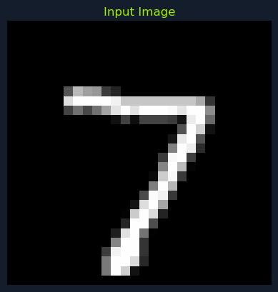
The first convolutional layer focuses on low-level features such as edges and borders. For example, it might detect the vertical and horizontal edges that form the digit "7".
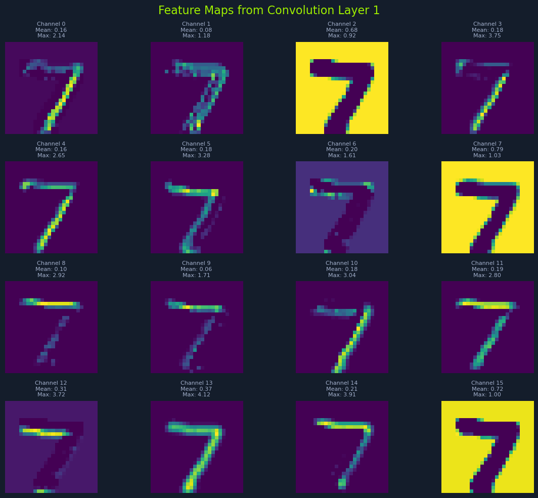
In this image, you can clearly see a focus on the border and edges of the number 7. The filter has highlighted the sharp transitions in intensity, which correspond to the boundaries of the digit.
The second convolutional layer builds upon the features extracted by the first layer. It combines these edge detections to identify more complex patterns, such as the interior structure of the digit.
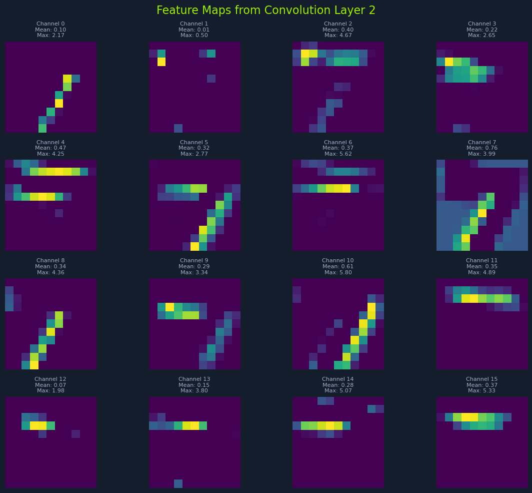
Here, you can see a focus on the inside of the number 7, rather than just the edges. The filter has detected the continuous lines and curves that form the digit, providing a more detailed representation.
This hierarchical feature extraction allows CNNs to represent complex visual information in a structured and efficient manner. By building upon the features learned in earlier layers, deeper layers can capture increasingly abstract and meaningful representations of the input data. This is why CNNs are so effective at tasks that require understanding complex visual scenes, such as image classification, object detection, and segmentation.
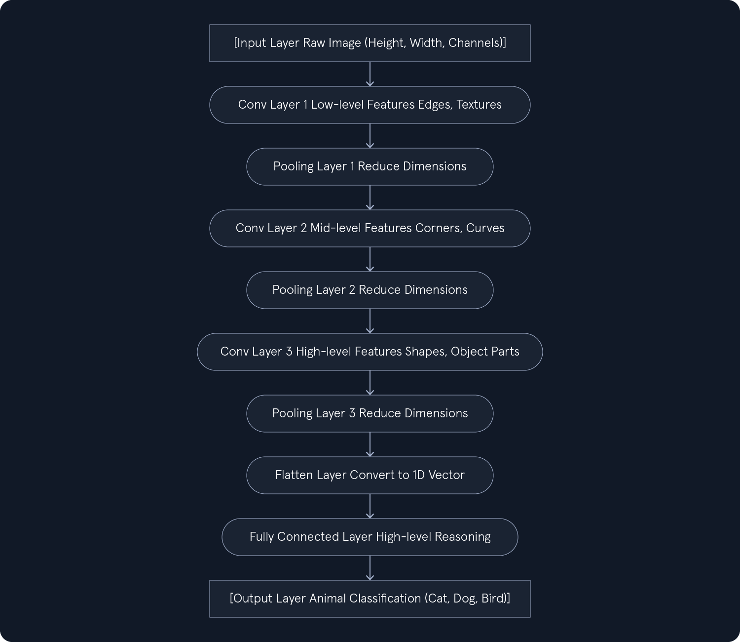
To illustrate this process, consider an image recognition task where a CNN is trained to classify images of different animals:
Input Layer: The input is a raw image, typically represented as a 3D tensor (height, width, channels).Convolutional Layers:Layer 1: Detects low-level features like edges and simple textures.Layer 2: Combines these features to detect more complex patterns, such as corners and curves.Layer 3: Recognizes higher-level structures like shapes and object parts.Pooling Layers:Fully Connected Layers:By stacking these layers, CNNs can learn to recognize complex visual patterns and make accurate predictions. This hierarchical structure is key to their success in various computer vision tasks.
While Convolutional Neural Networks (CNNs) have proven to be powerful tools for image recognition and other computer vision tasks, their effectiveness relies on certain assumptions about the input data. Understanding these assumptions is crucial for ensuring optimal performance and avoiding potential pitfalls.
CNNs are inherently designed to work with data structured as grids. This grid-like organization is fundamental to how CNNs process information. Common examples include:
Images: Represented as 2D grids, where each grid cell holds a pixel value. The dimensions typically include height, width, and channels (e.g., red, green, blue).Videos: Represented as 3D grids, extending the image concept by adding a time dimension. This results in a height, width, time, and channel structure.The grid structure is crucial because it allows CNNs to leverage localized convolutional operations, which we'll discuss later.
CNNs operate under the assumption that features within the data are organized hierarchically. This means that:
Lower-level features like edges, corners, or textures are simple and localized. They are typically captured in the network's early layers.Higher-level features are more complex and abstract, built upon these lower-level features. They represent larger patterns, shapes, or even entire objects and are detected in the deeper layers of the network.This hierarchical feature extraction is a defining characteristic of CNNs, enabling them to learn increasingly complex representations of the input data.
CNNs exploit the principle of feature locality, which assumes that relevant relationships between data points are primarily confined to local neighborhoods. For instance:
Another important assumption is feature stationarity, which implies that the meaning or significance of a feature remains consistent regardless of its location within the input data.
Effective training of CNNs relies on two practical considerations:
Sufficient data: CNNs, like most deep learning models, are data-hungry. They require large, labeled datasets to learn complex patterns and generalize to unseen data. Insufficient data can lead to overfitting, where the model performs well on training data but poorly on new data.Normalized input: Input data should be normalized to a standard range (e.g., scaling pixel values to between 0 and 1, or -1 and 1). This ensures stable and efficient training by preventing large variations in input values from disrupting the learning process.Adhering to these assumptions has proven remarkably successful in various tasks, including image classification, object detection, and natural language processing. Understanding these assumptions is crucial for designing, training, and deploying effective CNN models.
Recurrent Neural Networks (RNNs) are a class of artificial neural networks specifically designed to handle sequential data, where the order of the data points matters. Unlike traditional feedforward neural networks, which process data in a single pass, RNNs have a unique structure that allows them to maintain a "memory" of past inputs. This memory enables them to capture temporal dependencies and patterns within sequences, making them well-suited for tasks like natural language processing, speech recognition, and time series analysis.
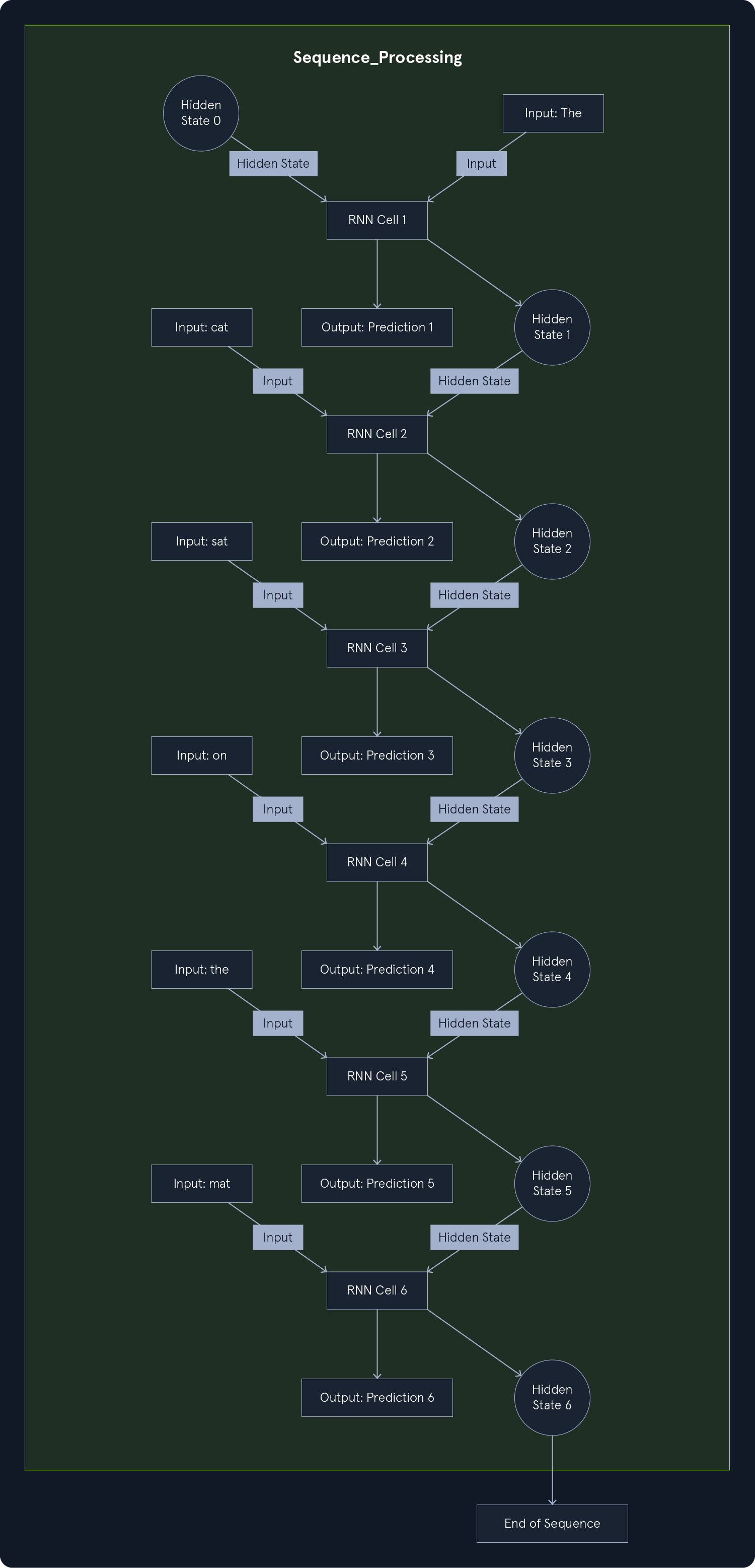
The key to understanding how RNNs handle sequential data lies in their recurrent connections. These connections create loops within the network, allowing information to persist and be passed from one step to the next. Imagine an RNN processing a sentence word by word. As it encounters each word, it considers the current input and incorporates information from the previous words, effectively "remembering" the context.
This process can be visualized as a chain of repeating modules, each representing a time step in the sequence. At each step, the module takes two inputs:
The module then performs calculations and produces two outputs:
This cyclical flow of information allows the RNN to learn patterns and dependencies across the entire sequence, enabling it to understand context and make informed predictions.
For example, consider the sentence, "The cat sat on the mat." An RNN processing this sentence would:
By the time the RNN reaches the word "mat," its hidden state would contain information about the entire preceding sentence, allowing it to make a more accurate prediction about what might come next.
While RNNs excel at processing sequential data, they can suffer from a significant challenge known as the vanishing gradient problem. This problem arises during training, specifically when using backpropagation through time (BPTT) to update the network's weights.
In BPTT, the gradients of the loss function are calculated and propagated back through the network to adjust the weights and improve the model's performance. However, as the gradients travel back through the recurrent connections, they can become increasingly smaller, eventually vanishing to near zero. This vanishing gradient hinders the network's ability to learn long-term dependencies, as the weights associated with earlier inputs receive minimal updates.
The vanishing gradient problem is particularly pronounced in RNNs due to the repeated multiplication of gradients across time steps. If the gradients are small (less than 1), their product diminishes exponentially as they propagate back through the network. This means that the influence of earlier inputs on the final output becomes negligible, limiting the RNN's ability to capture long-range dependencies.
To address the vanishing gradient problem, researchers have developed specialized RNN architectures, namely Long-Short-Term Memory (LSTM) and Gated Recurrent Unit (GRU) networks. These architectures introduce gating mechanisms that control the flow of information through the network, allowing them to better capture long-term dependencies.
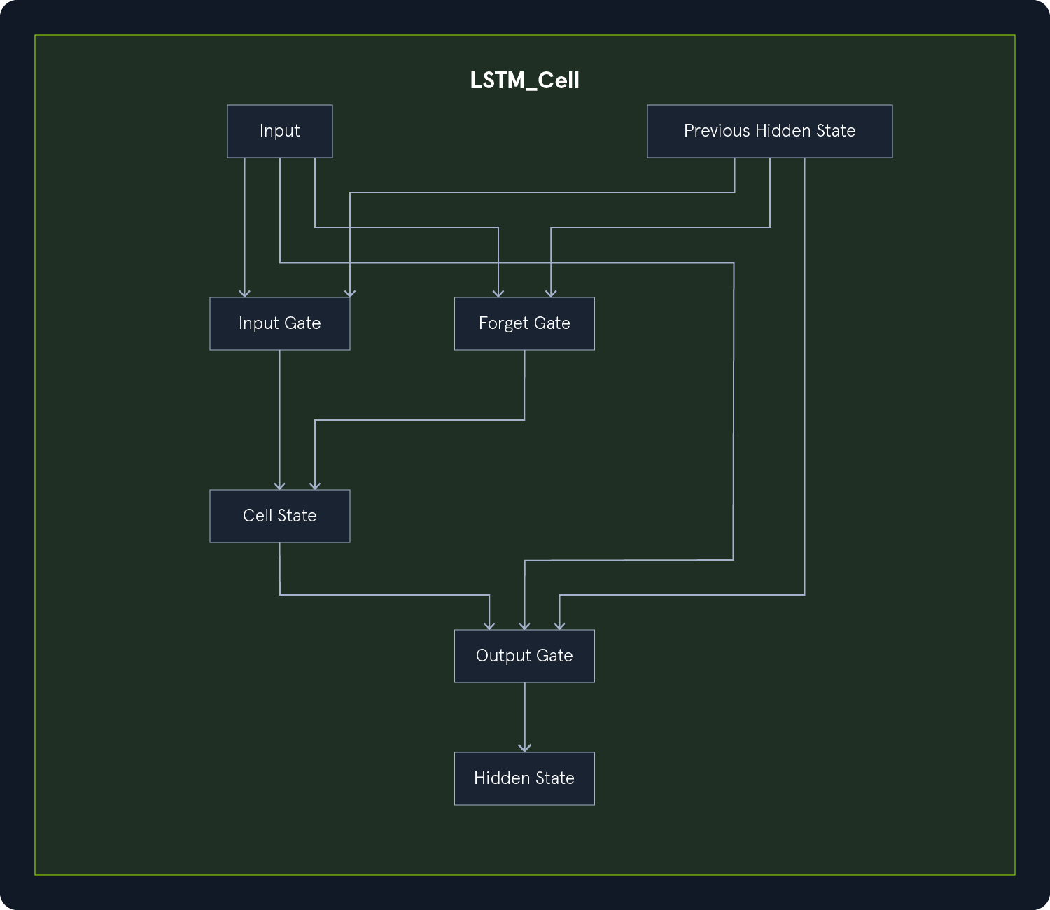
LSTMs incorporate memory cells that can store information over extended periods. These cells are equipped with three gates:
Input gate: Regulates the flow of new information into the memory cell.Forget gate: Controls how much of the existing information in the memory cell is retained or discarded.Output gate: Determines what information from the memory cell is output to the next time step.These gates enable LSTMs to selectively remember or forget information, mitigating the vanishing gradient problem and allowing them to learn long-term dependencies.
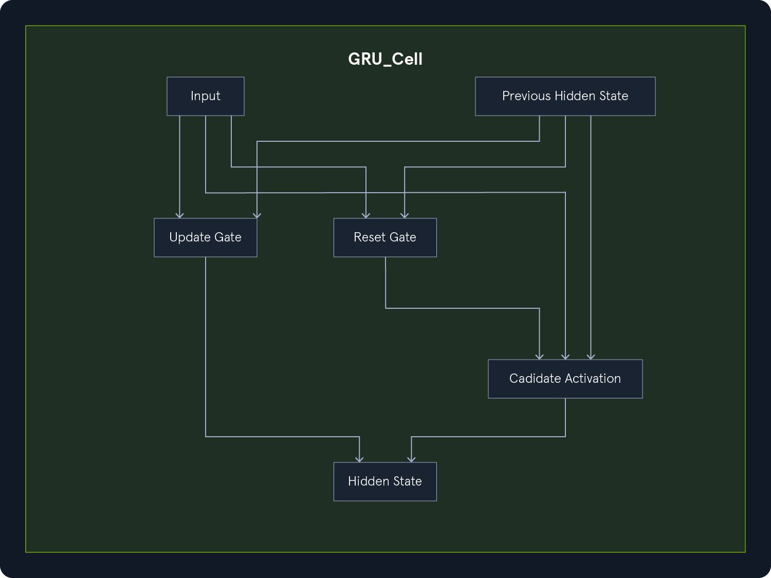
GRUs offer a simpler alternative to LSTMs, with only two gates:
Update gate: Controls how much of the previous hidden state is retained.Reset gate: Determines how much of the previous hidden state is combined with the current input.GRUs achieve comparable performance to LSTMs in many tasks while being computationally more efficient due to their reduced complexity.
LSTMs and GRUs have proven highly effective in overcoming the vanishing gradient problem, leading to significant advancements in sequence modeling tasks, including machine translation, speech recognition, and sentiment analysis.
In addition to the standard RNNs that process sequences in a forward direction, there are also bidirectional RNNs. These networks process the sequence in both forward and backward directions simultaneously. This allows them to capture information from past and future contexts, which can be beneficial in tasks where the entire sequence is available, such as natural language processing.
A bidirectional RNN consists of two RNNs, one processing the sequence from left to right and the other from right to left. The hidden states of both RNNs are combined at each time step to produce the final output. This approach enables the network to consider the entire context surrounding each element in the sequence, leading to improved performance in many tasks.
Generative AI represents a fascinating and rapidly evolving field within Machine Learning focused on creating new content or data that resembles human-generated output. Unlike traditional AI systems designed to recognize patterns, classify data, or make predictions, Generative AI focuses on producing original content, ranging from text and images to music and code.
Imagine an artist using their skills and imagination to create a painting. Similarly, Generative AI models leverage their learned knowledge to generate new and creative outputs, often exhibiting surprising originality and realism.
At the core of Generative AI lie complex algorithms, often based on neural networks, that learn a given dataset's underlying patterns and structures. This learning process allows the model to capture the data's statistical properties, enabling it to generate new samples that exhibit similar characteristics.
The process typically involves:
Training: The model is trained on a large dataset of examples, such as text, images, or music. During training, the model learns the statistical relationships between different elements in the data, capturing the patterns and structures that define the data's characteristics.Generation: Once trained, the model can generate new content by sampling from the learned distribution. This involves starting with a random seed or input and iteratively refining it based on the learned patterns until a satisfactory output is produced.Evaluation: The generated content is often evaluated based on its quality, originality, and resemblance to human-generated output. This evaluation can be subjective, relying on human judgment, or objective, using metrics that measure specific properties of the generated content.Various types of Generative AI models have been developed, each with its strengths and weaknesses:
Generative Adversarial Networks (GANs): GANs consist of two neural networks, a generator and a discriminator, that compete against each other. The generator creates new samples, while the discriminator distinguishes between real and generated samples. This adversarial process pushes both networks to improve, leading to increasingly realistic generated content.Variational Autoencoders (VAEs): VAEs learn a compressed data representation and use it to generate new samples. They are particularly effective in capturing the underlying structure of the data, allowing for a more controlled and diverse generation.Autoregressive Models: These models generate content sequentially, one element at a time, based on the previous elements. They are commonly used for text generation, generating each word based on the preceding words.Diffusion Models: These models gradually add noise to the data until it becomes pure noise. They then learn to reverse this process, generating new samples by starting from noise and refining it.Generative AI involves a unique set of concepts that are crucial for understanding how these models learn, generate content, and are evaluated. Let's explore some of the most important ones:
The latent space is a hidden representation of the data that captures its essential features and relationships in a compressed form. Think of it as a map where similar data points are clustered closer together, and dissimilar data points are further apart. Models like Variational Autoencoders (VAEs) learn a latent space to generate new content by sampling from this compressed representation.
Sampling is the process of generating new content by drawing from the learned distribution. It involves selecting values for the variables in the latent space and then mapping those values to the output space (e.g., generating an image from a point in the latent space). The quality and diversity of the generated content depend on how effectively the model has learned the underlying distribution and how well the sampling process captures the variations in that distribution.
Mode Collapse occurs when the generator learns to produce only a limited variety of outputs, even though the training data may contain a much wider range of possibilities. This can result in a lack of diversity in the generated content, with the generator getting stuck in a "mode" and failing to explore other modes of data distribution.
Overfitting is a common challenge in Machine Learning and applies to Generative AI. It occurs when the model learns the training data too well, capturing even the noise and irrelevant details. This can lead to poor generalization, where the model struggles to generate new content that differs significantly from the training examples. In Generative AI, overfitting can limit the model's creativity and originality.
Evaluating the quality and diversity of generated content is crucial in Generative AI. Various metrics have been developed for this purpose, each focusing on different aspects of the generated output. Some common evaluation metrics include:
Inception Score (IS): This score measures the quality and diversity of generated images by assessing their clarity and the diversity of the predicted classes.Fréchet Inception Distance (FID): Compares the distribution of generated images to the distribution of real images, with lower FID scores indicating greater similarity and better quality.BLEU score (for text generation): Measures the similarity between generated text and reference text, assessing the fluency and accuracy of the generated language.These metrics provide quantitative measures of the generated content's quality and diversity, helping researchers and developers assess the performance of Generative AI models and guide further improvements.
Large language models (LLMs) are a type of artificial intelligence (AI) that has gained significant attention in recent years due to their ability to understand and generate human-like text. These models are trained on massive amounts of text data, allowing them to learn patterns and relationships in language. This knowledge enables them to perform various tasks, including translation, summarization, question answering, and creative writing.
LLMs are typically based on a deep learning architecture called transformers. Transformers are particularly well-suited for processing sequential data like text because they can capture long-range dependencies between words. This is achieved through self-attention, which allows the model to weigh the importance of different words in a sentence when processing it.
The training process of an LLM involves feeding it massive amounts of text data and adjusting the model's parameters to minimize the difference between its predictions and the actual text. This process is computationally expensive and requires specialized hardware like GPUs or TPUs.
LLMs typically demonstrate three characteristics:
Massive Scale: LLMs are characterized by their enormous size, often containing billions or even trillions of parameters. This scale allows them to capture the nuances of human language.Few-Shot Learning: LLMs can perform new tasks with just a few examples, unlike traditional machine learning models that require large labeled datasets.Contextual Understanding: LLMs can understand the context of a conversation or text, allowing them to generate more relevant and coherent responses.Large language models represent a significant leap in artificial intelligence, showcasing impressive capabilities in understanding and generating human language. To truly grasp their power and potential, exploring the technical intricacies that drive their functionality is essential.
| Concept | Description |
|---|---|
Transformer Architecture | A neural network design that processes entire sentences in parallel, making it faster and more efficient than traditional RNNs. |
Tokenization | The process of converting text into smaller units called tokens, which can be words, subwords, or characters. |
Embeddings | Numerical representations of tokens that capture semantic meaning, with similar words having embeddings closer together in a high-dimensional space. |
Encoders and Decoders | Components of transformers where encoders process input text to capture its meaning, and decoders generate output text based on the encoder's output. |
Self-Attention Mechanism | A mechanism that calculates attention scores between words, allowing the model to understand long-range dependencies in text. |
Training | LLMs are trained using massive amounts of text data and unsupervised learning, adjusting parameters to minimize prediction errors using gradient descent. |
At the heart of most LLMs lies the transformer architecture, a neural network design that revolutionized natural language processing. Unlike traditional recurrent neural networks (RNNs) that process text sequentially, transformers can process entire sentences in parallel, making them significantly faster and more efficient.
The key innovation of transformers is the self-attention mechanism. Self-attention allows the model to weigh the importance of different words in a sentence when processing it. Imagine you're reading a sentence like "The cat sat on the mat." Self-attention would allow the model to understand that "cat" and "sat" are closely related, while "mat" is less important to the meaning of "sat."
Before an LLM can process text, it needs to be converted into a format the model can understand. This is done through tokenization, where the text is broken down into smaller units called tokens. Tokens can be words, subwords, or even characters, depending on the specific model.
For example, the sentence "I love artificial intelligence" might be tokenized as:
Code: python
["I", "love", "artificial", "intelligence"]
Once the text is tokenized, each token is converted into a numerical representation called an embedding. Embeddings capture the semantic meaning of words, representing them as points in a high-dimensional space. Words with similar meanings will have embeddings that are closer together in this space.
For instance, the embeddings for "king" and "queen" would be closer together than the embeddings for "king" and "table."
Transformers consist of two main components: encoders and decoders. Encoders process the input text, capturing its meaning and relationships between words. Decoders use this information to generate output text, such as a translation or a summary.
In the context of LLMs, the encoder and decoder work together to understand and generate human-like text. The encoder processes the input text, and the decoder generates text based on the encoder's output.
Self-attention is the key mechanism that allows transformers to capture long-range dependencies in text. It works by calculating attention scores between each pair of words in a sentence. These scores indicate how much each word should "pay attention" to other words.
For example, in the sentence "The cat sat on the mat, which was blue," self-attention would allow the model to understand that "which" refers to "mat," even though they are several words apart.
LLMs are trained on massive amounts of text data, often using unsupervised learning. This means the model learns patterns and relationships in the data without explicit labels or instructions.
The training involves feeding the model text data and adjusting its parameters to minimize the difference between its predictions and the actual text. This is typically done using a variant of gradient descent, an optimization algorithm that iteratively adjusts the model's parameters to minimize a loss function.
Let's say we want to use an LLM to generate a story about a cat. We would provide the model with a prompt, such as "Once upon a time, there was a cat named Whiskers." The LLM would then use its knowledge of language and storytelling to generate the rest of the story, word by word.
The model would consider the context of the prompt and its knowledge of grammar, syntax, and semantics to generate coherent and engaging text. It might generate something like:
Code: txt
Once upon a time, there was a cat named Whiskers. Whiskers was a curious and adventurous cat, always exploring the world around him. One day, he ventured into the forest and stumbled upon a hidden village of mice...
This is just a simplified example, but it illustrates how LLMs can generate creative and engaging text based on a given prompt.
Diffusion models are a class of generative models that have gained significant attention for their ability to generate high-quality images. Unlike traditional generative models like Generative Adversarial Networks (GANs) and Variational Autoencoders (VAEs), diffusion models use noise addition and removal steps to learn the data distribution. This approach has proven effective in generating realistic images, audio, and other data types.

Diffusion models function by gradually adding noise to an input image and then learning to reverse this process to generate new images. However, when generating images based on a textual prompt, such as "a cat in a hat," additional steps are required to incorporate the text into the generation process.
To generate an image from a textual prompt, diffusion models typically integrate a text encoder, such as a Transformer or CLIP, to convert the text into a latent representation. This latent representation then conditions the denoising process, ensuring the generated image aligns with the prompt.
Text Encoding: The first step is to encode the textual prompt using a pre-trained text encoder. For example, the prompt "a cat in a hat" is converted into a high-dimensional vector that captures the semantic meaning of the text. This vector serves as a conditioning input for the diffusion model.Conditioning the Denoising Process: The latent representation of the text is used to condition the denoising network. During the reverse process, the denoising network predicts the noise to be removed and ensures that the generated image aligns with the textual prompt. This is achieved by modifying the loss function to include a term that measures the discrepancy between the generated image and the text embedding.Sampling Process: The sampling process begins with pure noise, as in unconditional diffusion models. However, at each step of the reverse process, the denoising network uses both the noisy image and the text embedding to predict the noise. This ensures that the generated image gradually evolves to match the textual description.Final Image Generation: After a sufficient number of denoising steps, the model produces a final image consistent with the given prompt. The iterative process of adding and removing noise, guided by the text embedding, helps the model generate high-quality images that accurately reflect the textual description.By integrating these steps, diffusion models can effectively generate images from textual prompts, making them powerful tools for text-to-image synthesis, creative content generation, and more. The ability to condition the generation process on text allows diffusion models to produce diverse and contextually relevant images, opening up a wide range of applications in fields like art, design, and content creation.
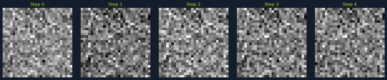
The forward process in diffusion models involves gradually adding noise to the data until it becomes pure noise. This process is often called the "forward diffusion" or "noising" process. Mathematically, this can be represented as:
Code: python
x_T = q(x_T | x_0)
Where:
x_0 is the original data (e.g., an image).x_T is the pure noise.q(x_T | x_0) is the distribution of the noisy data given the original data.A sequence of intermediate steps typically defines the forward process:
Code: python
x_t = q(x_t | x_{t-1})
Where:
t is the time step, ranging from 0 to T.q(x_t | x_{t-1}) is the transition probability from step t-1 to step t.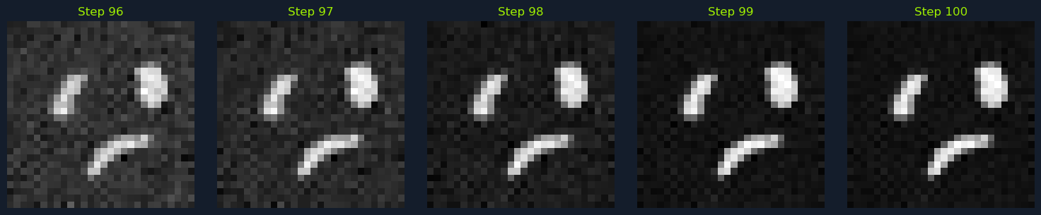
The reverse process, known as the "denoising" process, involves learning to remove the noise added during the forward process. The goal is to map the noisy data back to the original data distribution. This is achieved by training a neural network to predict the noise at each step:
Code: python
x_{t-1} = p_θ(x_{t-1} | x_t)
Where:
p_θ(x_{t-1} | x_t) is the learned distribution parameterized by the model's parameters θ.The reverse process is trained to minimize the difference between the predicted and actual noise added in the forward process. This is typically done using a loss function such as the mean squared error (MSE):
Code: python
L = E[||ε - ε_pred||^2]
Where:
ε is the actual noise.ε_pred is the predicted noise.
The noise schedule determines how much noise is added at each step of the forward process. A common choice is a linear schedule, where the variance of the noise increases linearly over time:
Code: python
β_t = β_min + (t / T) * (β_max - β_min)
Where:
β_t is the variance of the noise at step t.β_min and β_max are the minimum and maximum variances, respectively.The choice of the noise schedule can significantly impact the diffusion model's performance. A well-designed schedule ensures the model learns to denoise effectively across all time steps.
The denoising network is a neural network that learns to predict the noise at each time step. This network is typically a deep convolutional neural network (CNN) or a transformer, depending on the complexity of the data. The input to the network is the noisy data x_t, and the output is the predicted noise hat{ε}.
The architecture of the denoising network is crucial for the model's performance. It must be powerful enough to capture the complex patterns in the data and efficient enough to handle large datasets and high-resolution images.
Training a diffusion model involves minimizing the loss function over multiple time steps. This is done using gradient descent and backpropagation. The training process can be computationally intensive, especially for high-resolution images, but it results in a model that can generate high-quality samples.
The training process can be summarized as follows:
Initialize the Model: Start with an initial set of parameters θ for the denoising network.Forward Process: Add noise to the original data using the noise schedule.Reverse Process: Train the denoising network to predict the noise at each time step.Loss Calculation: Compute the loss between predicted and actual noise.Parameter Update: To minimize the loss, update the model parameters using gradient descent.Iterate: Repeat the process for multiple epochs until the model converges.
Once the model is trained, you can generate new images by sampling from the learned distribution. This involves starting with pure noise and iteratively applying the reverse process to remove the noise:
Code: python
x_0 = p_θ(x_0 | x_T)
Where:
x_T is the initial pure noise.p_θ(x_0 | x_T) is the learned distribution.The sampling process can be summarized as follows:
Start with Noise: Initialize the process with pure noise x_T.Iterative Denoising: For each time step t from T to 1, use the denoising network to predict the noise and update the data.Final Sample: After T steps, the resulting data x_0 is the generated image.Diffusion models make the following assumptions about the data:
Markov Property: The diffusion process exhibits the Markov property. This means that each step in both the forward (adding noise) and reverse (removing noise) processes depends only on the immediately preceding step, not the entire history of the process.Static Data Distribution: Diffusion models are trained on a fixed dataset, and they learn to represent the underlying distribution of this data. This data distribution is assumed to be static during training.Smoothness Assumption: While not a strict requirement, diffusion models often perform well when the data distribution is smooth. This means that small changes in the input data result in small changes in the output. This assumption helps the model learn the underlying structure of the data and generate realistic samples.