Following the Fundamentals of AI module, this module takes a more practical approach to applying machine learning techniques. Instead of focusing solely on theory, you will now engage in hands-on activities that involve building and evaluating real models. Throughout this process, you will gain experience with the end-to-end workflow of AI development, from exploring datasets to training and testing models.
You will construct three distinct AI models in this module:
Spam Classifier to determine whether an SMS message is spam or not.Network Anomaly Detection Model designed to identify abnormal or potentially malicious network traffic.Malware Classifier using byteplots, which are visual representations of binary data.Throughout the module, you will encounter python code blocks that guide you step-by-step through the model-building process.
You will learn more about Jupyter later in this module, but for now, understand that you can copy and paste these code snippets into a Jupyter notebook to execute them in sequence, either in the playground VM, or your environment.
You can train most of these models in your own environment. For a decent experience, you will need at least 4GB of RAM and at least 4 CPU cores.
Note: Throughout this module, all sections marked as interactive contain code blocks for you to follow along. Not all interactive sections contain separate exercises.
Setting up a proper environment is essential before diving into the exciting world of AI. This module offers two paths for an enviroment.
The first is The Playground. Because we acknowledge that not everyone will have the computer resources required to build the models in this module, we have provided a Virtual Playground Environment for you to use if you absolutely need it.
Because this is separate from PwnBox, there are specific sections where you can spawn this VM. You can connect to it using your HTB VPN profile or PwnBox. The VM exposes Jupyter for you to work in, which will be covered in the next section, but you can access it on http://<VM-IP>:8888. You can spawn the VM and extend instance time if needed at the bottom of this section or any of the Model Evaluation sections in the module.
:arrow-circle-left: :arrow-right: :redo: :home::bars:
Note: While the Playground environment is sufficient to follow along with everything discussed in this module, it lacks in performance to provide an environment that encourages experimentation. Therefore, we recommend setting up an environment on your own system, provided you have sufficiently powerful hardware. This will result in shorter training times and enable experimentation with different parameters, resulting in a more enjoyable way to work through the module and improve your understanding of the performance impact of different training parameters.
The second is to set up an environment on your own system, which you can do by following the rest of this section. For this module you will need at least 4GB of RAM. In a majority of cases, your own environment will provide faster training times than the playground VM.
Miniconda is a minimal installer for the Anaconda distribution of the Python programming language. It provides the conda package manager and a core Python environment without automatically installing the full suite of data science libraries available in Anaconda. Users can selectively install additional packages, creating a customized environment that aligns with their specific needs.
Both Miniconda and Anaconda rely on the conda package manager, allowing for simplified installation, updating, and management of Python packages and their dependencies. In essence, Miniconda offers a lighter starting point, while Anaconda comes pre-loaded with a broader range of commonly used data science tools.
You might wonder why we use Miniconda instead of a standard Python installation. Here are a few compelling reasons:
Performance: Miniconda often performs data science and machine learning tasks better due to optimized packages and libraries.Package Management: The Conda package manager simplifies package installation and management, ensuring compatibility and resolving dependencies. This is particularly crucial in deep learning, where projects often rely on a complex web of interconnected libraries.Environment Isolation: Miniconda allows you to create isolated environments for different projects. This prevents conflicts between packages and ensures each project has its dedicated dependencies.By using Miniconda, you'll streamline your workflow, avoid compatibility issues, and ensure that your deep learning environment is optimized for performance and efficiency.
While the traditional installer works well, we can streamline the process on Windows using Scoop, a command-line installer for Windows. Scoop simplifies the installation and management of various applications, including Miniconda.
First, install Scoop. Open PowerShell and run:
Environment Setup
C:\> Set-ExecutionPolicy RemoteSigned -scope CurrentUser # Allow scripts to run
C:\> irm get.scoop.sh | iex
Next, add the extras bucket, which contains Miniconda:
Environment Setup
C:\> scoop bucket add extras
Finally, install Miniconda with:
Environment Setup
C:\> scoop install miniconda3
This command installs the latest Python 3 version of Miniconda.
To verify the installation, close and reopen PowerShell. Type conda --version to check if Miniconda is installed correctly.
Environment Setup
C:\> conda --version

conda 24.9.2
Homebrew, a popular package manager for macOS, simplifies software installation and keeps it up-to-date. It also provides a convenient way for macOS users to install Miniconda.
If you don't have Homebrew, install it first by pasting the following command in your terminal:
Environment Setup
root@htb[/htb]$ /bin/bash -c "$(curl -fsSL https://raw.githubusercontent.com/Homebrew/install/HEAD/install.sh)"
Once Homebrew is set up, you can install Miniconda with this simple command:
Environment Setup
root@htb[/htb]$ brew install --cask miniconda
This command installs the latest version of Miniconda with Python 3.
To verify the installation, close and reopen your terminal. Type conda --version to confirm that Miniconda is installed correctly.
Environment Setup
root@htb[/htb]$ conda --version

conda 24.9.2
Miniconda provides a straightforward installation process that relies not solely on a distribution’s package manager. You can obtain the latest Miniconda installer directly from the official repository, run it silently, and then load the conda environment for your user shell. This approach ensures that conda commands and environments are readily available without manual configuration.
Environment Setup
root@htb[/htb]$ wget https://repo.anaconda.com/miniconda/Miniconda3-latest-Linux-x86_64.sh
root@htb[/htb]$ chmod +x Miniconda3-latest-Linux-x86_64.sh
root@htb[/htb]$ ./Miniconda3-latest-Linux-x86_64.sh -b -u
root@htb[/htb]$ eval "$(/home/$USER/miniconda3/bin/conda shell.$(ps -p $$ -o comm=) hook)"
Confirm that Miniconda is installed correctly by running:
Environment Setup
root@htb[/htb]$ conda --version

conda 24.9.2
The init command configures your shell to recognize and utilize conda. This step is essential for:
Activating environments: Allows you to use conda activate to switch between environments.Using conda commands: Ensures that conda commands are available in your shell.To initialize conda for your shell, run the following command after installing Miniconda:
Environment Setup
root@htb[/htb]$ conda init
This command will modify your shell configuration files (e.g., .bashrc or .zshrc) to include the necessary conda settings. You might need to close and reopen your terminal for the changes to take effect.
Finally, run these two commands to complete the init process
Environment Setup
root@htb[/htb]$ conda config --add channels defaults
root@htb[/htb]$ conda config --add channels conda-forge
root@htb[/htb]$ conda config --add channels nvidia # only needed if you are on a PC that has a nvidia gpu
root@htb[/htb]$ conda config --add channels pytorch
root@htb[/htb]$ conda config --set channel_priority strict
After installing Miniconda, you'll notice that the base environment is activated by default every time you open a new terminal. This is indicated by the (base) prefix on your path.
Environment Setup
(base) $
While this can be useful, it's often preferable to start with a clean slate and activate environments only when needed. Personally, I wouldn't say I like seeing the (base) prefix all the time, either.
To prevent the base environment from activating automatically, you can use the following command:
Environment Setup
root@htb[/htb]$ conda config --set auto_activate_base false
This command modifies the condarc configuration file and disables the automatic activation of the base environment.
When you open a new terminal, you won't see the (base) prefix in your prompt anymore.
In software development, managing dependencies can quickly become a complex task, especially when working on multiple projects with different library requirements.
This is where virtual environments come into play. A virtual environment is an isolated space where you can install packages and dependencies specific to a particular project, without interfering with other projects or your system's global Python installation.
They are critical for AI tasks for a few reasons:
Dependency Isolation: Each project can have its own set of dependencies, even if they conflict with those of other projects.Clean Project Structure: Keeps your project directory clean and organized by containing all dependencies within the environment.Reproducibility: Ensures that your project can be easily reproduced on different systems with the same dependencies.System Stability: Prevents conflicts with your global Python installation and avoids breaking other projects.conda provides a simple way to create virtual environments. For example, to create a new environment named ai with Python 3.11, use the following command:
Environment Setup
root@htb[/htb]$ conda create -n ai python=3.11
This will create a virtual environment, ai, which can then be used to contain all ai-related packages.
To activate the myenv environment, use:
Environment Setup
root@htb[/htb]$ conda activate ai
You'll notice that your terminal prompt now includes the environment name in parentheses (ai), indicating that the environment is active. Any packages you install using conda or pip will now be installed within this environment.
To deactivate the environment, use:
Environment Setup
root@htb[/htb]$ conda deactivate
The environment name will disappear from your prompt, and you'll be back to your base Python environment.
With your Miniconda environment set up, you can install the essential packages for your AI journey. These packages generally cover what will be needed in this module.
While conda provides a broad range of packages through its curated channels, it may not include every tool you require. In such cases, you can still use pip within the conda environment. This approach ensures you can install any additional packages that conda does not cover.
Use the conda install command to install the following core packages:
Environment Setup
root@htb[/htb]$ conda install -y numpy scipy pandas scikit-learn matplotlib seaborn transformers datasets tokenizers accelerate evaluate optimum huggingface_hub nltk category_encoders
root@htb[/htb]$ conda install -y pytorch torchvision torchaudio pytorch-cuda=12.4 -c pytorch -c nvidia
root@htb[/htb]$ pip install requests requests_toolbelt
conda provides a method to keep conda-managed packages up to date. Running the following command updates all conda-installed packages within the (ai) environment, but it does not update packages installed with pip. Any pip-installed packages must be managed separately, and mixing pip and conda installations may increase the risk of dependency conflicts.
Environment Setup
root@htb[/htb]$ conda update --all
JupyterLab is an interactive development environment that provides web-based coding, data, and visualization interfaces. Due to its flexibility and interactive features, it's a popular choice for data scientists and machine learning practitioners.
Interactive Environment: JupyterLab allows running code in individual cells, facilitating experimentation and iterative development.Data Exploration and Visualization: It integrates seamlessly with libraries like matplotlib and seaborn for creating visualizations and exploring data.Documentation and Sharing: JupyterLab supports markdown and LaTeX for creating rich documentation and sharing code with others.JupyterLab can be easily installed using conda, if it isn't already installed:
JupyterLab
root@htb[/htb]$ conda install -y jupyter jupyterlab notebook ipykernel
Make sure you are running the command from within your ai environment.
To start JupyterLab, simply run:
JupyterLab
root@htb[/htb]$ jupyter lab
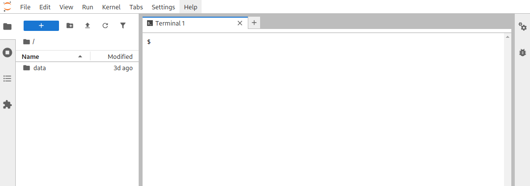
This will open a new tab in your web browser with the JupyterLab interface.
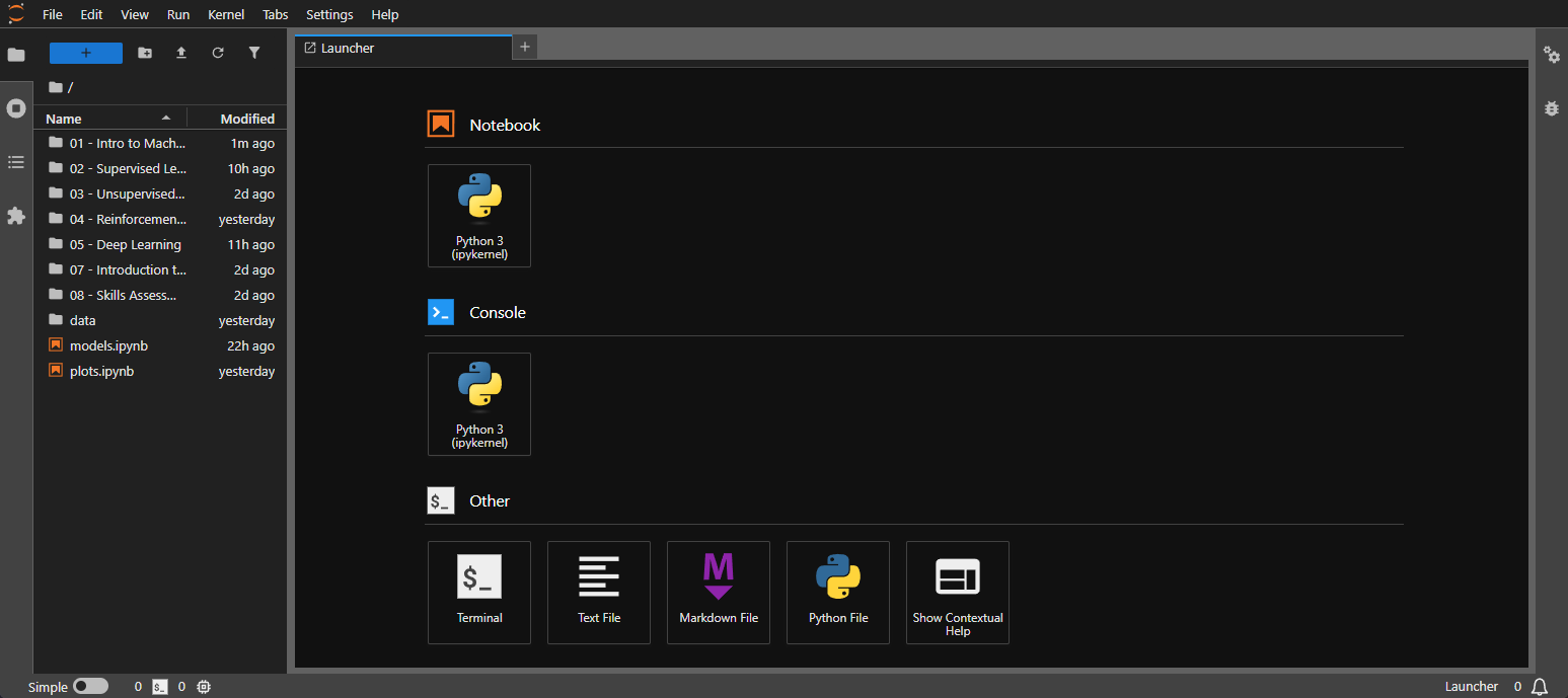
JupyterLab's primary component is the notebook, which allows combining code, text, and visualizations in a single document. Notebooks are organized into cells, where each cell can contain either code or markdown text.
Code cells: Execute code in various languages (Python, R, Julia).Markdown cells: Create formatted text, equations, and images using markdown syntax.Raw cells: Untyped raw text.Click the "Python 3" icon under the "Notebook" section in the Launcher interface to create a new notebook. This will open a notebook with a single empty code cell.
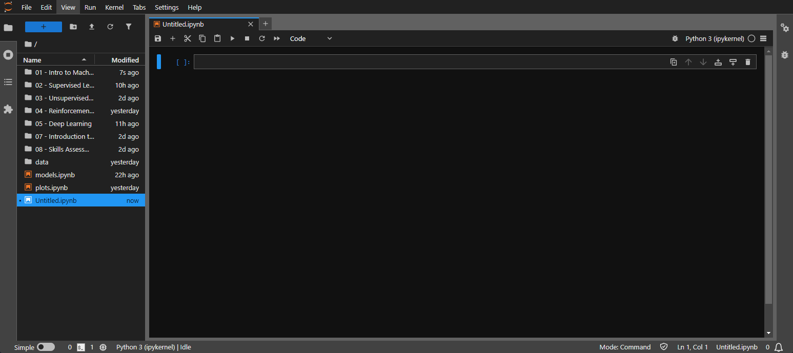
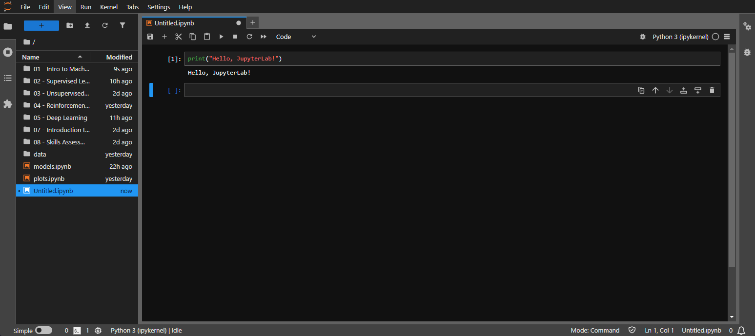
Type your Python code into the code cell and press Shift + Enter to execute it. For example:
Code: python
print("Hello, JupyterLab!")
The output of the code will appear below the cell.
Jupyter notebooks use a stateful environment, which means that variables, functions, and imports defined in one cell remain available to all later cells. Once you execute a cell, any changes it makes to the environment, such as assigning new variables or redefining functions, persist as long as the kernel is running. This differs from a stateless model, where each code execution is isolated and does not retain information from previous executions.
Being aware of the stateful nature of a notebook is important. For example, if you execute cells out of order, you might observe unexpected results due to previously defined or modified variables. Similarly, re-importing modules or updating variable values affects subsequent cell executions, but not those that were previously run.
Say you have a cell that does this:
Code: python
x = 1
then in a later cell you might have:
Code: python
print(x) # This will print '1' because 'x' was defined previously.
If you change the first cell to:
Code: python
x = 2
and re-run it before running the print(x) cell, the value of x in the environment becomes 2, so the output will now be different when you run the print cell.
Click the "+" button in the toolbar to add new cells. You can choose between code cells and markdown cells using the Dropdown on the toolbar. Markdown cells allow you to write formatted text and include headings, lists, and links.
JupyterLab integrates with libraries like pandas, matplotlib, and seaborn for data exploration and visualization. Here's an example of loading a dataset with pandas and creating a simple plot:
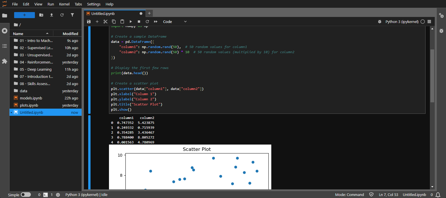
Code: python
import pandas as pd
import matplotlib.pyplot as plt
import numpy as np

# Create a sample DataFrame
data = pd.DataFrame({
    "column1": np.random.rand(50),  # 50 random values for column1
    "column2": np.random.rand(50) * 10  # 50 random values (multiplied by 10) for column2
})

# Display the first few rows
print(data.head())

# Create a scatter plot
plt.scatter(data["column1"], data["column2"])
plt.xlabel("Column 1")
plt.ylabel("Column 2")
plt.title("Scatter Plot")
plt.show()
This code now generates a sample DataFrame with two columns, column1 and column2, containing random values. The rest of the code remains the same, demonstrating how to display the DataFrame's contents and create a scatter plot using the generated data.
To save your notebook, click the save icon in the toolbar or use the Ctrl + S shortcut. Don't forget to rename your Notebook. You can right-click on the Notebook tab or the Notebook in the file browser.
JupyterLab uses a kernel to run your code. The kernel is a separate process responsible for executing code and maintaining the state of your computations. Sometimes, you may need to reset your environment if it becomes cluttered with variables or you encounter unexpected behavior.
Restarting the kernel clears all variables, functions, and imported modules from memory, allowing you to start fresh without shutting down JupyterLab entirely.
To restart the kernel:
Kernel menu in the top toolbar.Restart Kernel to reset the environment while preserving cell outputs, or Restart Kernel and Clear All Outputs to also remove all previously generated outputs from the notebook.After restarting, re-run any cells containing variable definitions, imports, or computations to restore the environment. This ensures that the notebook state accurately reflects the code you have most recently executed.
This is just a brief overview of Jupyter to get you up and running for this module. For an in-depth guide, refer to the JupyerLab Documentation.
Python is a versatile programming language widely used in Artificial Intelligence (AI) due to its rich library ecosystem that provides efficient and user-friendly tools for developing AI applications. This section focuses on two prominent Python libraries for AI development: Scikit-learn and PyTorch.
Just a quick note. This section provides a high-level overview of key Python libraries for AI, aiming to familiarize you with their purpose, structure, and common use cases. It offers a foundation for identifying relevant APIs and understanding the general landscape of these libraries. The official documentation will be your best resource to learning every small detail about the libraries. You do not need to copy and run these code snippets.
Scikit-learn is a comprehensive library built on NumPy, SciPy, and Matplotlib. It offers a wide range of algorithms and tools for machine learning tasks and provides a consistent and intuitive API, making implementing various machine learning models easy.
Supervised Learning: Scikit-learn provides a vast collection of supervised learning algorithms, including:Linear RegressionLogistic RegressionSupport Vector Machines (SVMs)Decision TreesNaive BayesEnsemble Methods (e.g., Random Forests, Gradient Boosting)Unsupervised Learning: It also offers various unsupervised learning algorithms, such as:Clustering (K-Means, DBSCAN)Dimensionality Reduction (PCA, t-SNE)Model Selection and Evaluation: Scikit-learn includes tools for model selection, hyperparameter tuning, and performance evaluation, enabling developers to optimize their models effectively.Data Preprocessing: It provides functionalities for data preprocessing, including:Scikit-learn offers a rich set of tools for preprocessing data, a crucial step in preparing data for machine learning algorithms. These tools help transform raw data into a suitable format that improves the accuracy and efficiency of models.
Feature scaling is essential to ensure that all features have a similar scale, preventing features with larger values from dominating the learning process. Scikit-learn provides various scaling techniques:
StandardScaler : Standardizes features by removing the mean and scaling to unit variance.MinMaxScaler : Scales features to a given range, typically between 0 and 1.RobustScaler : Scales features using statistics that are robust to outliers.Code: python
from sklearn.preprocessing import StandardScaler

scaler = StandardScaler()
X_scaled = scaler.fit_transform(X)
Categorical features, representing data in categories or groups, need to be converted into numerical representations for machine learning algorithms to process them. Scikit-learn offers encoding techniques:
OneHotEncoder : Creates binary (0 or 1) columns for each category.LabelEncoder : Assigns a unique integer to each category.Code: python
from sklearn.preprocessing import OneHotEncoder

encoder = OneHotEncoder()
X_encoded = encoder.fit_transform(X)
Real-world datasets often contain missing values. Scikit-learn provides methods to handle these missing values:
SimpleImputer : Replaces missing values with a specified strategy (e.g., mean, median, most frequent).KNNImputer : Imputes missing values using the k-Nearest Neighbors algorithm.Code: python
from sklearn.impute import SimpleImputer

imputer = SimpleImputer(strategy='mean')
X_imputed = imputer.fit_transform(X)
Scikit-learn offers tools for selecting the best model and evaluating its performance.
Splitting data into training and testing sets is crucial to evaluating the model's generalization ability to unseen data.
Code: python
from sklearn.model_selection import train_test_split

X_train, X_test, y_train, y_test = train_test_split(X, y, test_size=0.2)
Cross-validation provides a more robust evaluation by splitting the data into multiple folds and training/testing on different combinations.
Code: python
from sklearn.model_selection import cross_val_score

scores = cross_val_score(model, X, y, cv=5)
Scikit-learn provides various metrics to evaluate model performance:
accuracy_score : For classification tasks.mean_squared_error : For regression tasks.precision_score, recall_score, f1_score : For classification tasks with imbalanced classes.Code: python
from sklearn.metrics import accuracy_score

accuracy = accuracy_score(y_test, y_pred)
Scikit-learn follows a consistent API for training and predicting with different models.
Create an instance of the desired model with appropriate hyperparameters.
Code: python
from sklearn.linear_model import LogisticRegression

model = LogisticRegression(C=1.0)
Train the model using the fit() method with the training data.
Code: python
model.fit(X_train, y_train)
Make predictions on new data using the predict() method.
Code: python
y_pred = model.predict(X_test)
PyTorch is an open-source machine learning library developed by Facebook's AI Research lab. It provides a flexible and powerful framework for building and deploying various types of machine learning models, including deep learning models.
Deep Learning: PyTorch excels in deep learning, enabling the development of complex neural networks with multiple layers and architectures.Dynamic Computational Graphs: Unlike static computational graphs used in libraries like TensorFlow, PyTorch uses dynamic computational graphs, which allow for more flexible and intuitive model building and debugging.GPU Support: PyTorch supports GPU acceleration, significantly speeding up the training process for computationally intensive models.TorchVision Integration: TorchVision is a library integrated with PyTorch that provides a user-friendly interface for image datasets, pre-trained models, and common image transformations.Automatic Differentiation: PyTorch uses autograd to automatically compute gradients, simplifying the process of backpropagation.Community and Ecosystem: PyTorch has a large and active community, leading to a rich ecosystem of tools, libraries, and resources.At the heart of PyTorch lies the concept of dynamic computational graphs. A dynamic computational graph is created on the fly during the forward pass, allowing for more flexible and dynamic model building. This makes it easier to implement complex and non-linear models.
Tensors are multi-dimensional arrays that hold the data being processed. They can be constants, variables, or placeholders. PyTorch tensors are similar to NumPy arrays but can run on GPUs for faster computation.
Code: python
import torch

# Creating a tensor
x = torch.tensor([1.0, 2.0, 3.0])

# Tensors can be moved to GPU if available
if torch.cuda.is_available():
    x = x.to('cuda')
PyTorch provides a flexible and intuitive interface for building and training deep learning models. The torch.nn module contains various layers and modules for constructing neural networks.
The Sequential API allows building models layer by layer, adding each layer sequentially.
Code: python
import torch.nn as nn

model = nn.Sequential(
    nn.Linear(784, 128),
    nn.ReLU(),
    nn.Linear(128, 10),
    nn.Softmax(dim=1)
)
The Module class provides more flexibility for building complex models with non-linear topologies, shared layers, and multiple inputs/outputs.
Code: python
import torch.nn as nn

class CustomModel(nn.Module):
    def __init__(self):
        super(CustomModel, self).__init__()
        self.layer1 = nn.Linear(784, 128)
        self.relu = nn.ReLU()
        self.layer2 = nn.Linear(128, 10)
        self.softmax = nn.Softmax(dim=1)

    def forward(self, x):
        x = self.layer1(x)
        x = self.relu(x)
        x = self.layer2(x)
        x = self.softmax(x)
        return x

model = CustomModel()
PyTorch provides tools for training and evaluating models.
Optimizers are algorithms that adjust the model's parameters during training to minimize the loss function. PyTorch offers various optimizers:
AdamSGD (Stochastic Gradient Descent)RMSpropCode: python
import torch.optim as optim

optimizer = optim.Adam(model.parameters(), lr=0.001)
Loss Functions measure the difference between the model's predictions and the actual target values. PyTorch provides a variety of loss functions:
CrossEntropyLoss : For multi-class classification.BCEWithLogitsLoss : For binary classification.MSELoss : For regression.Code: python
import torch.nn as nn

loss_fn = nn.CrossEntropyLoss()
Metrics evaluate the model's performance during training and testing.
AccuracyPrecisionRecallCode: python
def accuracy(output, target):
    _, predicted = torch.max(output, 1)
    correct = (predicted == target).sum().item()
    return correct / len(target)
The training loop updates the model's parameters based on the training data.
Code: python
import torch

epochs = 10
num_batches = 100

for epoch in range(epochs):
    for batch in range(num_batches):
        # Get batch of data
        x_batch, y_batch = get_batch(batch)

        # Forward pass
        y_pred = model(x_batch)

        # Calculate loss
        loss = loss_fn(y_pred, y_batch)

        # Backward pass and optimization
        optimizer.zero_grad()
        loss.backward()
        optimizer.step()

        # Optional: print loss or other metrics
        if batch % 10 == 0:
            print(f'Epoch [{epoch+1}/{epochs}], Batch [{batch+1}/{num_batches}], Loss: {loss.item():.4f}')
PyTorch provides the torch.utils.data.Dataset and DataLoader classes for handling data loading and preprocessing.
Code: python
from torch.utils.data import Dataset, DataLoader

class CustomDataset(Dataset):
    def __init__(self, data, labels):
        self.data = data
        self.labels = labels

    def __len__(self):
        return len(self.data)

    def __getitem__(self, idx):
        return self.data[idx], self.labels[idx]

# Example usage
dataset = CustomDataset(data, labels)
dataloader = DataLoader(dataset, batch_size=32, shuffle=True)
PyTorch allows models to be saved and loaded for inference or further training.
Code: python
# Save model
torch.save(model.state_dict(), 'model.pth')

# Load model
model = CustomModel()
model.load_state_dict(torch.load('model.pth'))
model.eval()  # Set the model to evaluation mode
In AI, the quality and characteristics of the data used to train models significantly impact their performance and accuracy. Datasets, which are collections of data points used for analysis and model training, come in various forms and formats, each with its own properties and considerations. Data preprocessing is a crucial step in the machine-learning pipeline that involves transforming raw data into a suitable format for algorithms to process effectively.
Datasets are structured collections of data used for analysis and model training. They come in various forms, including:
Tabular Data: Data organized into tables with rows and columns, common in spreadsheets or databases.Image Data: Sets of images represented numerically as pixel arrays.Text Data: Unstructured data composed of sentences, paragraphs, or full documents.Time Series Data: Sequential data points collected over time, emphasizing temporal patterns.The quality of a dataset is fundamental to the success of any data analysis or machine learning project. Here’s why:
Model Accuracy: High-quality datasets produce more accurate models. Poor-quality data—such as noisy, incomplete, or biased datasets—leads to reduced model performance.Generalization: Carefully curated datasets enable models to generalize effectively to unseen data. This minimizes overfitting and ensures consistent performance in real-world applications.Efficiency: Clean, well-prepared data reduces both training time and computational demands, streamlining the entire process.Reliability: Reliable datasets lead to trustworthy insights and decisions. In critical domains like healthcare or finance, data quality directly affects the dependability of results.Several key attributes characterize a good dataset:
| Attribute | Description | Example |
|---|---|---|
Relevance |
The data should be relevant to the problem at hand. Irrelevant data can introduce noise and reduce model performance. | Text data from social media posts is more relevant than stock market prices for a sentiment analysis task. |
Completeness |
The dataset should have minimal missing values. Missing data can lead to biased models and incorrect predictions. | Techniques like imputation can handle missing values, but it's best to start with a complete dataset if possible. |
Consistency |
Data should be consistent in format and structure. Inconsistencies can cause errors during preprocessing and model training. | Ensure that date formats are uniform across the dataset (e.g.,YYYY-MM-DD). |
Quality |
The data should be accurate and free from errors. Errors can arise from data collection, entry, or transmission issues. | Data validation and verification processes can help ensure data quality. |
Representativeness |
The dataset should be representative of the population it aims to model. A biased or unrepresentative dataset can lead to biased models. | A facial recognition system's dataset should include a diverse range of faces from different ethnicities, ages, and genders. |
Balance |
The dataset should be balanced, especially for classification tasks. Imbalanced datasets can lead to biased models that perform poorly on minority classes. | Techniques like oversampling, undersampling, or generating synthetic data can help balance the dataset. |
Size |
The dataset should be large enough to capture the complexity of the problem. Small datasets may not provide enough information for the model to learn effectively. | However, large datasets can also be computationally expensive and require more powerful hardware. |
The provided dataset, demo_dataset.csv is a CSV file containing network log entries. Each record describes a network event and includes details such as the source IP address, destination port, protocol used, the volume of data transferred, and an associated threat level. Analyzing these entries allows one to simulate various network scenarios that are useful for developing and evaluating intrusion detection systems.
The dataset consists of multiple columns, each serving a specific purpose:
log_id: Unique identifier for each log entry.source_ip: Source IP address for the network event.destination_port: Destination port number used by the event.protocol: Network protocol employed (e.g., TCP, TLS, SSH).bytes_transferred: Total bytes transferred during the event.threat_level: Indicator of the event's severity. 0 denotes normal traffic, 1 indicates low-threat activity, and 2 signifies a high-threat event.Before processing, it is essential to note potential difficulties:
threat_level column includes unknown values (e.g., ?, -1) that must be standardized or addressed during preprocessing.Acknowledging these challenges early allows the data to be properly cleaned and transformed, facilitating accurate and reliable analysis.
We first load it into a pandas DataFrame to begin working with the dataset. A pandas DataFrame is a flexible, two-dimensional labeled data structure that supports a variety of operations for data exploration and preprocessing. Key advantages include labeled axes, heterogeneous data handling, and integration with other Python libraries.
Utilizing a DataFrame simplifies subsequent tasks like inspection, cleaning, encoding, and data transformation.
Code: python
import pandas as pd

# Load the dataset
data = pd.read_csv("./demo_dataset.csv")
In this code, pd.read_csv("./demo_dataset.csv") loads the downloaded CSV file into a DataFrame named data. From here, inspecting, manipulating, and preparing the dataset for further steps in the analysis pipeline becomes straightforward.
After loading the dataset, we employ various operations to understand its structure, identify anomalies, and determine the nature of cleaning or transformations needed.
We examine the first few rows to get a quick overview, which can help detect obvious issues like unexpected column names, incorrect data types, or irregular patterns.
Code: python
# Display the first few rows of the dataset
print(data.head())
This command outputs the initial rows of the DataFrame, offering an immediate glimpse into the dataset's overall organization.
Understanding the data types and completeness of each column is essential. We can quickly review the dataset's information, including which columns have null values and the total number of entries per column.
Code: python
# Get a summary of column data types and non-null counts
print(data.info())
The info() method reveals the dataset's shape, column names, data types, and how many entries are present for each column, enabling early detection of columns with missing or unexpected data.
Missing values or anomalies must be handled to maintain the dataset's integrity. The next step is to identify how many missing values each column contains.
Code: python
# Identify columns with missing values
print(data.isnull().sum())
This command returns the count of null values for each column, helping to prioritize which features need attention. Addressing these missing values may involve imputation, removal, or other cleaning strategies to ensure the dataset remains reliable and valid for further analysis.
Data preprocessing transforms raw data into a suitable format for machine learning algorithms. Key techniques include:
Data Cleaning: Handling missing values, removing duplicates, and smoothing noisy data.Data Transformation: Normalizing, encoding, scaling, and reducing data.Data Integration: Merging and aggregating data from multiple sources.Data Formatting: Converting data types and reshaping data structures.Effective preprocessing addresses inconsistencies, missing values, outliers, noise, and feature scaling, improving the accuracy, efficiency, and robustness of machine learning models.
In addition to missing values, we need to check for invalid values in specific columns. Here are some common checks for the given dataset.
To identify invalid source_ip values, you can use a regular expression to validate the IP addresses:
Code: python
import re

def is_valid_ip(ip):
    pattern = re.compile(r'^((25[0-5]|2[0-4][0-9]|[01]?[0-9][0-9]?)\.){3}(25[0-5]|2[0-4][0-9]|[01]?[0-9][0-9]?)$')
    return bool(pattern.match(ip))

# Check for invalid IP addresses
invalid_ips = data[~data['source_ip'].astype(str).apply(is_valid_ip)]
print(invalid_ips)
To identify invalid destination_port values, you can check if the port numbers are within the valid range (0-65535):
Code: python
def is_valid_port(port):
    try:
        port = int(port)
        return 0 <= port <= 65535
    except ValueError:
        return False

# Check for invalid port numbers
invalid_ports = data[~data['destination_port'].apply(is_valid_port)]
print(invalid_ports)
To identify invalid protocol values, you can check against a list of known protocols:
Code: python
valid_protocols = ['TCP', 'TLS', 'SSH', 'POP3', 'DNS', 'HTTPS', 'SMTP', 'FTP', 'UDP', 'HTTP']

# Check for invalid protocol values
invalid_protocols = data[~data['protocol'].isin(valid_protocols)]
print(invalid_protocols)
To identify invalid bytes_transferred values, you can check if the values are numeric and non-negative:
Code: python
def is_valid_bytes(bytes):
    try:
        bytes = int(bytes)
        return bytes >= 0
    except ValueError:
        return False

# Check for invalid bytes transferred
invalid_bytes = data[~data['bytes_transferred'].apply(is_valid_bytes)]
print(invalid_bytes)
To identify invalid threat_level values, you can check if the values are within a valid range (e.g., 0-2):
Code: python
def is_valid_threat_level(threat_level):
    try:
        threat_level = int(threat_level)
        return 0 <= threat_level <= 2
    except ValueError:
        return False

# Check for invalid threat levels
invalid_threat_levels = data[~data['threat_level'].apply(is_valid_threat_level)]
print(invalid_threat_levels)
There are a few different ways we can approach this bad data.
The most straightforward approach is to discard the invalid entries entirely. This ensures that the remaining dataset is clean and free of potentially misleading information.
Code: python
# the ignore errors covers the fact that there might be some overlap between indexes that match other invalid criteria
data = data.drop(invalid_ips.index, errors='ignore')
data = data.drop(invalid_ports.index, errors='ignore')
data = data.drop(invalid_protocols.index, errors='ignore')
data = data.drop(invalid_bytes.index, errors='ignore')
data = data.drop(invalid_threat_levels.index, errors='ignore')

print(data.describe(include='all'))
This method is generally preferred when data accuracy is paramount, and the loss of some data points does not significantly compromise the overall analysis. However, it may not always be feasible, especially if the dataset is small or the invalid entries constitute a substantial portion of the data.
After dropping the bad data from our dataset, we are only left with 77 clean entries.
It is sometimes possible to clean or transform invalid entries into valid and usable data instead of discarding them. This approach aims to retain as much information as possible from the dataset.
Imputing is the process of replacing missing or invalid values in a dataset with estimated values. This is crucial for maintaining the integrity and usability of the data, especially in machine learning and data analysis tasks where missing values can lead to biased or inaccurate results.
First, convert all invalid or corrupted entries, such as MISSING_IP, INVALID_IP, STRING_PORT, UNUSED_PORT, NON_NUMERIC, or ?, into NaN. This approach standardizes the representation of missing values, enabling uniform downstream imputation steps.
Code: python
import pandas as pd
import numpy as np
import re
from ipaddress import ip_address

df = pd.read_csv('demo_dataset.csv')

invalid_ips = ['INVALID_IP', 'MISSING_IP']
invalid_ports = ['STRING_PORT', 'UNUSED_PORT']
invalid_bytes = ['NON_NUMERIC', 'NEGATIVE']
invalid_threat = ['?']

df.replace(invalid_ips + invalid_ports + invalid_bytes + invalid_threat, np.nan, inplace=True)

df['destination_port'] = pd.to_numeric(df['destination_port'], errors='coerce')
df['bytes_transferred'] = pd.to_numeric(df['bytes_transferred'], errors='coerce')
df['threat_level'] = pd.to_numeric(df['threat_level'], errors='coerce')

def is_valid_ip(ip):
    pattern = re.compile(r'^((25[0-5]|2[0-4][0-9]|[01]?\d?\d)\.){3}(25[0-5]|2[0-4]\d|[01]?\d?\d)$')
    if pd.isna(ip) or not pattern.match(str(ip)):
        return np.nan
    return ip

df['source_ip'] = df['source_ip'].apply(is_valid_ip)
After this step, NaN represents all missing or invalid data points.
For basic numeric columns like bytes_transferred, use simple methods such as the median or mean. For categorical columns like protocol, use the most frequent value.
Code: python
from sklearn.impute import SimpleImputer

numeric_cols = ['destination_port', 'bytes_transferred', 'threat_level']
categorical_cols = ['protocol']

num_imputer = SimpleImputer(strategy='median')
df[numeric_cols] = num_imputer.fit_transform(df[numeric_cols])

cat_imputer = SimpleImputer(strategy='most_frequent')
df[categorical_cols] = cat_imputer.fit_transform(df[categorical_cols])
These imputations ensure that all columns have valid, non-missing values, though they do not consider complex relationships among features.
For more sophisticated scenarios, employ advanced techniques like KNNImputer or IterativeImputer. These methods consider relationships among features to produce contextually meaningful imputations.
Code: python
from sklearn.impute import KNNImputer

knn_imputer = KNNImputer(n_neighbors=5)
df[numeric_cols] = knn_imputer.fit_transform(df[numeric_cols])
After cleaning and imputations, apply domain knowledge. For source_ip values that remain missing, assign a default such as 0.0.0.0. Validate protocol values against known valid protocols. For ports, ensure values fall within the valid range 0-65535, and for protocols that imply certain ports, consider mode-based assignments or domain-specific mappings.
Code: python
valid_protocols = ['TCP', 'TLS', 'SSH', 'POP3', 'DNS', 'HTTPS', 'SMTP', 'FTP', 'UDP', 'HTTP']
df.loc[~df['protocol'].isin(valid_protocols), 'protocol'] = df['protocol'].mode()[0]

df['source_ip'] = df['source_ip'].fillna('0.0.0.0')
df['destination_port'] = df['destination_port'].clip(lower=0, upper=65535)
Perform final verification steps to confirm that distributions are reasonable and categorical sets remain valid. Adjust imputation strategies and transformations or remove problematic records if anomalies persist.
Code: python
print(df.describe(include='all'))
Data transformations improve the representation and distribution of features, making them more suitable for machine learning models. These transformations ensure that models can efficiently capture underlying patterns by converting categorical variables into machine-readable formats and addressing skewed numerical distributions. They also enhance trained models' stability, interpretability, and predictive performance.
Encoding converts categorical values into numeric form so machine learning algorithms can utilize these features. Depending on the situation, you can choose:
OneHotEncoder for binary indicator features that represent each category separately.LabelEncoder for integer codes, though this may imply unintended order.HashingEncoder or frequency-based methods to handle high-cardinality features and control feature space size.After encoding, verify that the transformed features are meaningful and do not introduce artificial ordering.
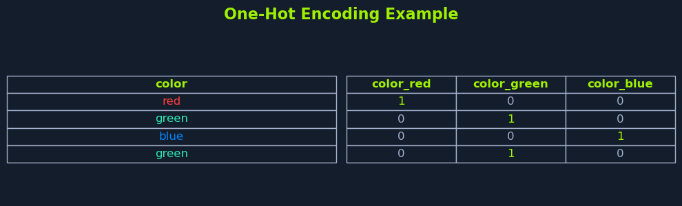
One-hot encoding takes a categorical feature and converts it into a set of new binary features, where each binary feature corresponds to one possible category value. This process creates a set of indicator columns that hold 1 or 0, indicating the presence or absence of a particular category in each row.
For example, consider the categorical feature color, which can take on the values red, green, or blue. In a dataset, you might have rows where color is red in one instance, green in another, and so on. By applying one-hot encoding, instead of keeping a single column with values like red, green, or blue, the encoding creates three new binary columns:
color_redcolor_greencolor_blueEach of these new columns corresponds to one of the original categories. If a row had color set to red, the color_red column for that row would be 1, and the other two columns (color_green and color_blue) would be 0. Similarly, if color was originally green, then the color_green column would be 1, while the color_red and color_blue columns would be 0.
This approach prevents models from misinterpreting category values as numeric hierarchies. However, it can increase the number of features if a category has many unique values.
In this case, we are going to encode the protocol feature.
Code: python
from sklearn.preprocessing import OneHotEncoder

encoder = OneHotEncoder(handle_unknown='ignore', sparse_output=False)
encoded = encoder.fit_transform(df[['protocol']])

encoded_df = pd.DataFrame(encoded, columns=encoder.get_feature_names_out(['protocol']))
df = pd.concat([df.drop('protocol', axis=1), encoded_df], axis=1)
The original protocol feature is replaced with distinct binary columns, ensuring the model interprets each category independently.
When a feature is skewed, its values are unevenly distributed, often with most observations clustered near one end and a few extreme values stretching out the distribution. Such skew can affect the performance of machine learning models, especially those sensitive to outliers or that assume more uniform or normal-like data distributions.
Scaling or transforming these skewed features helps models better capture patterns in the data. One common transformation is applying a log transform to compress large values more than small ones, resulting in a more balanced distribution and less dominated by outliers. By doing this, models often gain improved stability, accuracy, and generalization ability.
Below, we show how to apply a log transform using the log1p function. This approach adds 1 to each value before taking the log, ensuring that the transform is defined even for values at or near zero.
Code: python
import numpy as np

# Apply logarithmic transformation to a skewed feature to reduce its skewness
df["bytes_transferred"] = np.log1p(df["bytes_transferred"])  # Add 1 to avoid log(0)
The code above transforms the bytes_transferred feature. Before this transformation, the feature might have had a few very large values, overshadowing the majority of smaller observations. After the transformation, the distribution is evener, helping the model treat all data points fairly and reducing the risk of overfitting outliers.
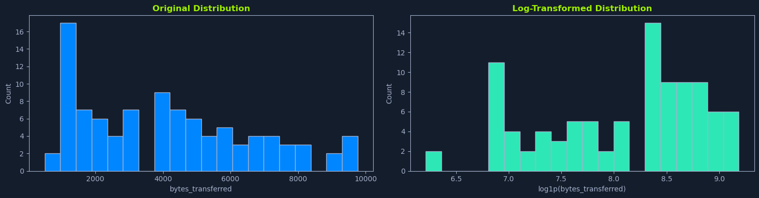
Visual comparisons of the distribution before and after the transform (as shown by the above figure) confirm that the original skew has been substantially reduced. Although no information is lost, the model now views the data through a lens that downplays extreme cases and highlights underlying patterns more clearly.
Data splitting involves dividing a dataset into three distinct subsets—training, validation, and testing—to ensure reliable model evaluation. By having separate sets, you can train your model on one subset, fine-tune it on another, and finally test its performance on data it has never seen before.
Training Set: Used to fit the model. Typically accounts for around 60-80% of the entire dataset.Validation Set: Used for tuning hyperparameters and model selection. Often around 10-20% of the entire dataset.Test Set: Used only after all model selections and tuning are complete. Often around 10-20% of the entire dataset.The code below demonstrates one approach using train_test_split from scikit-learn. The initial split allocates 80% of the data for training and 20% for testing. A subsequent split divides the 80% training portion into 60% for final training and 20% for validation.
Note that test_size=0.25 in the second split refers to 25% of the previously created training subset (which is 80% of the data). In other words, 0.8 × 0.25 = 0.2 (20% of the entire dataset), leaving 60% for training and 20% for validation overall.
Code: python
from sklearn.model_selection import train_test_split

# Separate features (X) and target (y)
X = df.drop("threat_level", axis=1)
y = df["threat_level"]

# Initial split: 80% training, 20% testing
X_train, X_test, y_train, y_test = train_test_split(X, y, test_size=0.2, random_state=1337)

# Second split: from the 80% training portion, allocate 60% for final training and 20% for validation
X_train, X_val, y_train, y_val = train_test_split(X_train, y_train, test_size=0.25, random_state=1337)
These subsets support a structured workflow:
X_train and y_train.X_val and y_val.X_test and y_test.When assessing a trained machine learning model, one examines a set of numerical metrics to gauge how well the model performs on a given task. These metrics often quantify the relationship between predictions and known ground-truth labels.
In the Fundamentals of AI module, we briefly covered metrics such as accuracy, precision, recall, and F1-score, and we know that these metrics provide different perspectives on model behavior.
Accuracy is the proportion of correct predictions out of all predictions made. It measures how often the model classifies instances correctly. A model with accuracy: 0.9950 indicates that it makes correct predictions 99.50% of the time.
Key points about accuracy:
(true positives + true negatives) / (all instances).While accuracy appears intuitive, relying on it alone can hide important details. Consider a spam classification scenario where only 1% of incoming emails are spam and 99% are legitimate. A model that always predicts every email as legitimate will achieve accuracy: 0.99, but it will never catch any spam.
In this case, accuracy fails to highlight the model’s inability to correctly identify the minority class. This underscores the importance of complementary metrics, such as precision, recall, or F1-score, which provide a more nuanced understanding of performance when dealing with imbalanced datasets.
Precision measures how often the model’s predicted positives are truly positive. For precision: 0.9949, when the model labels an instance as positive, it is correct 99.49% of the time.
Key points about precision:
true positives / (true positives + false positives).precision reduces wasted effort caused by false alarms.With the spam classification example, if the model labels 100 emails as spam, and 99 of them are actually spam, then its precision is high. This reduces the inconvenience of losing important, legitimate emails to the spam folder. However, if the model rarely identifies spam in the first place, it may fail to catch a large portion of malicious emails. High precision alone does not guarantee that the model is finding all the spam it should.
Recall measures the model’s ability to identify all positive instances. For recall: 0.9950, the model detects 99.50% of all positives.
Key points about recall:
true positives / (true positives + false negatives).recall reduces the risk of missing critical cases.In the spam classification scenario, a model with high recall correctly flags most spam emails. This helps ensure that suspicious content does not slip through unnoticed. However, a model with very high recall but low precision might flood the spam folder with benign emails. Although it rarely misses spam, it inconveniences the user by misclassifying too many legitimate emails as spam.
F1-score is the harmonic mean of precision and recall. For F1-score: 0.9949, the metric indicates a near-perfect balance between these two aspects.
Key points about F1-score:
precision and recall.2 * (precision * recall) / (precision + recall).Continuing with the spam classification scenario, the F1-score ensures that the model not only minimizes the misclassification of legitimate emails (high precision) but also effectively identifies the majority of spam messages (high recall). By focusing on the balance rather than just one metric, the F1-score provides a more complete picture of the model’s performance in identifying and correctly handling both spam and non-spam emails.
While these four metrics are common, other measures may provide further insights:
Specificity: Measures how effectively the model identifies negatives.AUC: The Area Under the ROC Curve, indicating the model’s discriminative capability at various thresholds.Matthews Correlation Coefficient: Useful for highly imbalanced datasets.Confusion Matrix: Summarizes predictions versus true labels, offering a comprehensive view of performance.Such metrics and visualizations help confirm that the given high values truly reflect robust performance, not just favorable conditions in the dataset.
When evaluating a model’s metrics (accuracy: 0.9750, precision: 0.9300, recall: 0.9100, F1-score: 0.9200), consider the following:
Even metrics that look impressive may not fully capture real-world performance if the dataset does not reflect operational conditions. For instance, high accuracy could be achieved if negative cases are heavily overrepresented, making it easier to appear correct by default. Verifying that both precision and recall remain robust helps ensure the model identifies important instances without becoming overwhelmed by incorrect predictions.
Depending on the setting, certain trade-offs emerge:
recall to avoid missing critical threats, even if it occasionally flags benign events.precision can reduce the burden caused by following up on false alarms.These metrics, considered together, provide a balanced perspective. The relatively high and reasonably aligned precision and recall values yield a strong F1-score, suggesting that the model performs consistently well across different classes. This balanced performance supports confidence that the model’s decisions are both reliable and meaningful in practice.
Spam, or unsolicited bulk messaging, has been a persistent issue since the early days of digital communication. It clutters inboxes, poses security risks, and can be used for malicious purposes such as phishing attacks. Effective spam detection is crucial for maintaining the integrity and usability of email systems and other messaging platforms.
Bayes' Theorem is a fundamental concept in probability theory that describes the probability of an event based on prior knowledge of conditions that might be related to the event. Mathematically, it is expressed as:
Code: python
P(A|B) = (P(B|A) * P(A)) / P(B)
Where:
P(A|B) is the probability of event A occurring, given that B is true.P(B|A) is the probability of event B occurring, given that A is true.P(A) is the prior probability of event A.P(B) is the prior probability of event B.In the context of spam detection, A can represent the hypothesis that an email is spam (Spam), and B can represent the observed features of the email (e.g., words, phrases, etc.).
Let's break down how Bayes' Theorem can be applied to determine if an email is spam:
Hypothesis: We want to determine the probability that an email is spam given its features.P(Spam|Features): Probability that an email is spam given its features.Likelihood: This is the probability of observing the features given that the email is spam.P(Features|Spam): Probability of the features appearing in a spam email.Prior Probability: The probability that any email is spam, irrespective of its features.P(Spam): Prior probability of an email being spam.Marginal Likelihood: The total probability of observing the features, considering both spam and non-spam emails.P(Features): Probability of the features appearing in any email.Using Bayes' Theorem, we can express this as:
Code: python
P(Spam|Features) = (P(Features|Spam) * P(Spam)) / P(Features)
Naive Bayes makes the "naive" assumption that the presence of a particular feature in an email is independent of the presence of any other feature, given the class label. This simplifies the calculation of P(Features|Spam):
Code: python
P(Features|Spam) = P(feature1|Spam) * P(feature2|Spam) * ... * P(featureN|Spam)
Similarly, for non-spam emails:
Code: python
P(Features|Not Spam) = P(feature1|Not Spam) * P(feature2|Not Spam) * ... * P(featureN|Not Spam)
Using these probabilities, we can calculate the posterior probability of an email being spam or not spam given its features. The class with the higher posterior probability is chosen as the predicted class.
Suppose we have an email with features F1 and F2. We want to determine if this email is spam.
P(Spam) = 0.3: Prior probability that any email is spam.P(Not Spam) = 0.7: Prior probability that any email is not spam.P(F1|Spam) = 0.4: Probability of feature F1 given the email is spam.P(F2|Spam) = 0.5: Probability of feature F2 given the email is spam.P(F1|Not Spam) = 0.2: Probability of feature F1 given the email is not spam.P(F2|Not Spam) = 0.3: Probability of feature F2 given the email is not spam.Using the Naive Bayes assumption:
Code: python
P(F1, F2|Spam) = P(F1|Spam) * P(F2|Spam) = 0.4 * 0.5 = 0.2
P(F1, F2|Not Spam) = P(F1|Not Spam) * P(F2|Not Spam) = 0.2 * 0.3 = 0.06
Now, applying Bayes' Theorem:
Code: python
P(Spam|F1, F2) = (P(F1, F2|Spam) * P(Spam)) / P(F1, F2)
To find P(F1, F2), we use the law of total probability:
Code: python
P(F1, F2) = P(F1, F2|Spam) * P(Spam) + P(F1, F2|Not Spam) * P(Not Spam)
          = (0.2 * 0.3) + (0.06 * 0.7)
          = 0.06 + 0.042
          = 0.102
Thus:
Code: python
P(Spam|F1, F2) = (0.2 * 0.3) / 0.102
               = 0.06 / 0.102
               ≈ 0.588
Similarly:
Code: python
P(Not Spam|F1, F2) = (P(F1, F2|Not Spam) * P(Not Spam)) / P(F1, F2)
                   = (0.06 * 0.7) / 0.102
                   = 0.042 / 0.102
                   ≈ 0.412
Since P(Spam|F1, F2) > P(Not Spam|F1, F2), the email is classified as spam.
We'll explore Bayesian spam classification using the SMS Spam Collection dataset, a curated resource tailored for developing and evaluating text-based spam filters. This dataset emerges from the combined efforts of Tiago A. Almeida and Akebo Yamakami at the School of Electrical and Computer Engineering at the University of Campinas in Brazil, and José María Gómez Hidalgo at the R\&D Department of Optenet in Spain.
Their work, "Contributions to the Study of SMS Spam Filtering: New Collection and Results," presented at the 2011 ACM Symposium on Document Engineering, aimed to address the growing problem of unsolicited mobile phone messages, commonly known as SMS spam. Recognizing that many existing spam filtering resources focused on email rather than text messages, the authors assembled this dataset from multiple sources, including the Grumbletext website, the NUS SMS Corpus, and Caroline Tag’s PhD thesis.
The resulting corpus contains 5,574 text messages annotated as either ham (legitimate) or spam (unwanted), making it a great resource for building and testing models that can differentiate meaningful communications from intrusive or deceptive ones. In this context, ham refers to messages from known contacts, subscriptions, or newsletters that hold value for the recipient, while spam represents unsolicited content that typically offers no benefit and may even pose risks to the user.
The first step in our process is to download this dataset, and we'll do it programmatically in our notebook.
Code: python
import requests
import zipfile
import io

# URL of the dataset
url = "https://archive.ics.uci.edu/static/public/228/sms+spam+collection.zip"
# Download the dataset
response = requests.get(url)
if response.status_code == 200:
    print("Download successful")
else:
    print("Failed to download the dataset")
We use the requests library to send an HTTP GET request to the URL of the dataset. We check the status code of the response to determine if the download was successful (status_code == 200).
After downloading the dataset, we need to extract its contents. The dataset is provided in a .zip file format, which we will handle using Python's zipfile and io libraries.
Code: python
# Extract the dataset
with zipfile.ZipFile(io.BytesIO(response.content)) as z:
    z.extractall("sms_spam_collection")
    print("Extraction successful")
Here, response.content contains the binary data of the downloaded .zip file. We use io.BytesIO to convert this binary data into a bytes-like object that can be processed by zipfile.ZipFile. The extractall method extracts all files from the archive into a specified directory, in this case, sms_spam_collection.
It's useful to verify that the extraction was successful and to see what files were extracted.
Code: python
import os

# List the extracted files
extracted_files = os.listdir("sms_spam_collection")
print("Extracted files:", extracted_files)
The os.listdir function lists all files and directories in the specified path, allowing us to confirm that the SMSSpamCollection file is present.
With the dataset extracted, we can now load it into a pandas DataFrame for further analysis. The SMS Spam Collection dataset is stored in a tab-separated values (TSV) file format, which we specify using the sep parameter in pd.read_csv.
Code: python
import pandas as pd

# Load the dataset
df = pd.read_csv(
    "sms_spam_collection/SMSSpamCollection",
    sep="\t",
    header=None,
    names=["label", "message"],
)
Here, we specify that the file is tab-separated (sep="\t"), and since the file does not contain a header row, we set header=None and provide column names manually using the names parameter.
After loading the dataset, it is important to inspect it for basic information, missing values, and duplicates. This helps ensure that the data is clean and ready for analysis.
Code: python
# Display basic information about the dataset
print("-------------------- HEAD --------------------")
print(df.head())
print("-------------------- DESCRIBE --------------------")
print(df.describe())
print("-------------------- INFO --------------------")
print(df.info())
To get an overview of the dataset, we can use the head, describe, and info methods provided by pandas.
df.head() displays the first few rows of the DataFrame, giving us a quick look at the data.df.describe() provides a statistical summary of the numerical columns in the DataFrame. Although our dataset is primarily text-based, this can still be useful for understanding the distribution of labels.df.info() gives a concise summary of the DataFrame, including the number of non-null entries and the data types of each column.Checking for missing values is crucial to ensure that our dataset does not contain any incomplete entries.
Code: python
# Check for missing values
print("Missing values:\n", df.isnull().sum())
The isnull method returns a DataFrame of the same shape as the original, with boolean values indicating whether each entry is null. The sum method then counts the number of True values in each column, giving us the total number of missing entries.
Duplicate entries can skew the results of our analysis, so it's important to identify and remove them.
Code: python
# Check for duplicates
print("Duplicate entries:", df.duplicated().sum())

# Remove duplicates if any
df = df.drop_duplicates()
The duplicated method returns a boolean Series indicating whether each row is a duplicate or not. The sum method counts the number of True values, giving us the total number of duplicate entries. We then use the drop_duplicates method to remove these duplicates from the DataFrame.
After loading the SMS Spam Collection dataset, the next step is preprocessing the text data. Preprocessing standardizes the text, reduces noise, and extracts meaningful features, all of which improve the performance of the Bayes spam classifier. The steps outlined here rely on the nltk library for tasks such as tokenization, stop word removal, and stemming.
Before processing any text, you must download the required NLTK data files. These include punkt for tokenization and stopwords for removing common words that do not contribute to meaning. Ensuring all required resources are available at this stage prevents interruptions during later processing steps.
Code: python
import nltk

# Download the necessary NLTK data files
nltk.download("punkt")
nltk.download("punkt_tab")
nltk.download("stopwords")

print("=== BEFORE ANY PREPROCESSING ===")
print(df.head(5))
Lowercasing the text ensures that the classifier treats words equally, regardless of their original casing. By converting all characters to lowercase, the model considers "Free" and "free" as the same token, effectively reducing dimensionality and improving consistency.
Code: python
# Convert all message text to lowercase
df["message"] = df["message"].str.lower()
print("\n=== AFTER LOWERCASING ===")
print(df["message"].head(5))
After this step, the dataset contains uniformly cased text, preventing the model from assigning different weights to tokens that differ only by letter case.
Removing unnecessary punctuation and numbers simplifies the dataset by focusing on meaningful words. However, certain symbols such as $ and ! may contain important context in spam messages. For example, $ might indicate a monetary amount, and ! might add emphasis.
The code below removes all characters other than lowercase letters, whitespace, dollar signs, or exclamation marks. This balance between cleaning the data and preserving important symbols helps the model concentrate on features relevant to distinguishing spam from ham messages.
Code: python
import re

# Remove non-essential punctuation and numbers, keep useful symbols like $ and !
df["message"] = df["message"].apply(lambda x: re.sub(r"[^a-z\s$!]", "", x))
print("\n=== AFTER REMOVING PUNCTUATION & NUMBERS (except $ and !) ===")
print(df["message"].head(5))
After this step, the text is cleaner, more uniform, and better suited for subsequent preprocessing tasks such as tokenization, stop word removal, or stemming.
Tokenization divides the message text into individual words or tokens, a crucial step before further analysis. By converting unstructured text into a sequence of words, we prepare the data for operations like removing stop words and applying stemming. Each token corresponds to a meaningful unit, allowing downstream processes to operate on smaller, standardized elements rather than entire sentences.
Code: python
from nltk.tokenize import word_tokenize

# Split each message into individual tokens
df["message"] = df["message"].apply(word_tokenize)
print("\n=== AFTER TOKENIZATION ===")
print(df["message"].head(5))
Once tokenized, the dataset contains messages represented as lists of words, ready for additional preprocessing steps that further refine the text data.
Stop words are common words like and, the, or is that often do not add meaningful context. Removing them reduces noise and focuses the model on the words most likely to help distinguish spam from ham messages. By reducing the number of non-informative tokens, we help the model learn more efficiently.
Code: python
from nltk.corpus import stopwords

# Define a set of English stop words and remove them from the tokens
stop_words = set(stopwords.words("english"))
df["message"] = df["message"].apply(lambda x: [word for word in x if word not in stop_words])
print("\n=== AFTER REMOVING STOP WORDS ===")
print(df["message"].head(5))
The token lists are shorter at this stage and contain fewer non-informative words, setting a cleaner stage for future text transformations.
Stemming normalizes words by reducing them to their base form (e.g., running becomes run). This consolidates different forms of the same root word, effectively cutting the vocabulary size and smoothing out the text representation. As a result, the model can better understand the underlying concepts without being distracted by trivial variations in word forms.
Code: python
from nltk.stem import PorterStemmer

# Stem each token to reduce words to their base form
stemmer = PorterStemmer()
df["message"] = df["message"].apply(lambda x: [stemmer.stem(word) for word in x])
print("\n=== AFTER STEMMING ===")
print(df["message"].head(5))
After stemming, the token lists focus on root word forms, further simplifying the text and improving the model’s generalization ability.
While tokens are useful for manipulation, many machine-learning algorithms and vectorization techniques (e.g., TF-IDF) work best with raw text strings. Rejoining the tokens into a space-separated string restores a format compatible with these methods, allowing the dataset to move seamlessly into the feature extraction phase.
Code: python
# Rejoin tokens into a single string for feature extraction
df["message"] = df["message"].apply(lambda x: " ".join(x))
print("\n=== AFTER JOINING TOKENS BACK INTO STRINGS ===")
print(df["message"].head(5))
At this point, the messages are fully preprocessed. Each message is a cleaned, normalized string ready for vectorization and subsequent model training, ultimately improving the classifier’s performance.
Feature extraction transforms preprocessed SMS messages into numerical vectors suitable for machine learning algorithms. Since models cannot directly process raw text data, they rely on numeric representations—such as counts or frequencies of words—to identify patterns that differentiate spam from ham.
A common way to represent text numerically is through a bag-of-words model. This technique constructs a vocabulary of unique terms from the dataset and represents each message as a vector of term counts. Each element in the vector corresponds to a term in the vocabulary, and its value indicates how often that term appears in the message.
Using only unigrams (individual words) does not preserve the original word order; it treats each document as a collection of terms and their frequencies, independent of sequence.
To introduce a limited sense of order, we also include bigrams, which are pairs of consecutive words. By incorporating bigrams, we capture some local ordering information.
For example, the bigram free prize might help distinguish a spam message promising a reward from a simple statement containing the word free alone. However, beyond these small sequences, the global order of words and sentence structure remains largely lost. In other words, CountVectorizer does not preserve complete word order; it only captures localized patterns defined by the chosen ngram_range.
CountVectorizer from the scikit-learn library efficiently implements the bag-of-words approach. It converts a collection of documents into a matrix of term counts, where each row represents a message and each column corresponds to a term (unigram or bigram). Before transformation, CountVectorizer applies tokenization, builds a vocabulary, and then maps each document to a numeric vector.
Key parameters for refining the feature set:
min_df=1: A term must appear in at least one document to be included. While this threshold is set to 1 here, higher values can be used in practice to exclude rare terms.max_df=0.9: Terms that appear in more than 90% of the documents are excluded, removing overly common words that provide limited differentiation.ngram_range=(1, 2): The feature matrix captures individual words and common word pairs by including unigrams and bigrams, potentially improving the model’s ability to detect spam patterns.Code: python
from sklearn.feature_extraction.text import CountVectorizer

# Initialize CountVectorizer with bigrams, min_df, and max_df to focus on relevant terms
vectorizer = CountVectorizer(min_df=1, max_df=0.9, ngram_range=(1, 2))

# Fit and transform the message column
X = vectorizer.fit_transform(df["message"])

# Labels (target variable)
y = df["label"].apply(lambda x: 1 if x == "spam" else 0)  # Converting labels to 1 and 0
After this step, X becomes a numerical feature matrix ready to be fed into a classifier, such as Naive Bayes.
CountVectorizer operates in three main stages:
Tokenization: Splits the text into tokens based on the specified ngram_range. For ngram_range=(1, 2), it extracts both unigrams (like "message") and bigrams (like "free prize").Building the Vocabulary: Uses min_df and max_df to decide which terms to include. Terms that are too rare or common are filtered out, leaving a vocabulary that balances informative and distinctive terms.Vectorization: Transforms each document into a vector of term counts. Each vector entry corresponds to a term from the vocabulary, and its value represents how many times that term appears in the document.Consider five documents:
The free prize is waiting for youThe spam message offers a free prize nowThe spam filter might detect thisThe important news says you won a free tripThe message truly is importantIf we use ngram_range=(1, 1) (unigrams only) and min_df=1, max_df=0.9, the word The will be removed from unigram vocabulary by max_df=0.9 since it appears more than 90% in the documents, leaving the below unigram matrix:
| Document | free | prize | is | waiting | for | you | spam | message | offers | a | now | filter | might | detect | this | important | news | says | won | trip | truly |
|---|---|---|---|---|---|---|---|---|---|---|---|---|---|---|---|---|---|---|---|---|---|
| 1 | 1 | 1 | 1 | 1 | 1 | 1 | 0 | 0 | 0 | 0 | 0 | 0 | 0 | 0 | 0 | 0 | 0 | 0 | 0 | 0 | 0 |
| 2 | 1 | 1 | 0 | 0 | 0 | 0 | 1 | 1 | 1 | 1 | 1 | 0 | 0 | 0 | 0 | 0 | 0 | 0 | 0 | 0 | 0 |
| 3 | 0 | 0 | 0 | 0 | 0 | 0 | 1 | 0 | 0 | 0 | 0 | 1 | 1 | 1 | 1 | 0 | 0 | 0 | 0 | 0 | 0 |
| 4 | 1 | 0 | 0 | 0 | 0 | 1 | 0 | 0 | 0 | 1 | 0 | 0 | 0 | 0 | 0 | 1 | 1 | 1 | 1 | 1 | 0 |
| 5 | 0 | 0 | 1 | 0 | 0 | 0 | 0 | 1 | 0 | 0 | 0 | 0 | 0 | 0 | 0 | 1 | 0 | 0 | 0 | 0 | 1 |
Using ngram_range=(1, 2), the final vocabulary includes all of the above unigrams and any valid bigrams containing those unigrams. For instance, free prize occurs in Documents 1 and 2. The resulting matrix provides additional context, helping the model differentiate messages more effectively:
| Document | free | prize | is | waiting | for | you | spam | message | offers | a | now | filter | might | detect | this | important | news | says | won | trip | truly | free prize | prize is | is waiting | waiting for | for you | spam message | message offers | offers a | a free | prize now | spam filter | filter might | might detect | detect this | important news | news says | says you | you won | won a | free trip | message truly | truly is | is important |
|---|---|---|---|---|---|---|---|---|---|---|---|---|---|---|---|---|---|---|---|---|---|---|---|---|---|---|---|---|---|---|---|---|---|---|---|---|---|---|---|---|---|---|---|---|
| 1 | 1 | 1 | 1 | 1 | 1 | 1 | 0 | 0 | 0 | 0 | 0 | 0 | 0 | 0 | 0 | 0 | 0 | 0 | 0 | 0 | 0 | 1 | 1 | 1 | 1 | 1 | 0 | 0 | 0 | 0 | 0 | 0 | 0 | 0 | 0 | 0 | 0 | 0 | 0 | 0 | 0 | 0 | 0 | 0 |
| 2 | 1 | 1 | 0 | 0 | 0 | 0 | 1 | 1 | 1 | 1 | 1 | 0 | 0 | 0 | 0 | 0 | 0 | 0 | 0 | 0 | 0 | 1 | 0 | 0 | 0 | 0 | 1 | 1 | 1 | 1 | 1 | 0 | 0 | 0 | 0 | 0 | 0 | 0 | 0 | 0 | 0 | 0 | 0 | 0 |
| 3 | 0 | 0 | 0 | 0 | 0 | 0 | 1 | 0 | 0 | 0 | 0 | 1 | 1 | 1 | 0 | 0 | 0 | 0 | 0 | 0 | 0 | 0 | 0 | 0 | 0 | 0 | 0 | 0 | 0 | 0 | 0 | 1 | 1 | 1 | 1 | 0 | 0 | 0 | 0 | 0 | 0 | 0 | 0 | 0 |
| 4 | 1 | 0 | 0 | 0 | 0 | 1 | 0 | 0 | 0 | 1 | 0 | 0 | 0 | 0 | 1 | 1 | 1 | 1 | 1 | 0 | 0 | 0 | 0 | 0 | 0 | 0 | 0 | 0 | 0 | 1 | 0 | 0 | 0 | 0 | 0 | 1 | 1 | 1 | 1 | 1 | 1 | 0 | 0 | 0 |
| 5 | 0 | 0 | 1 | 0 | 0 | 0 | 0 | 1 | 0 | 0 | 0 | 0 | 0 | 0 | 1 | 0 | 0 | 0 | 0 | 0 | 1 | 0 | 0 | 0 | 0 | 0 | 0 | 0 | 0 | 0 | 0 | 0 | 0 | 0 | 0 | 0 | 0 | 0 | 0 | 0 | 0 | 1 | 1 | 1 |
This feature extraction process, using CountVectorizer, has transformed our text data into a resulting matrix provides a concise, numerical representation of each message, ready for training a classification model.
After preprocessing the text data and extracting meaningful features, we train a machine-learning model for spam detection. We use the Multinomial Naive Bayes classifier, which is well-suited for text classification tasks due to its probabilistic nature and ability to efficiently handle large, sparse feature sets.
To streamline the entire process, we employ a Pipeline. A pipeline chains together the vectorization and modeling steps, ensuring that the same data transformation (in this case, CountVectorizer) is consistently applied before feeding the transformed data into the classifier. This approach simplifies both development and maintenance by encapsulating the feature extraction and model training into a single, unified workflow.
Code: python
from sklearn.model_selection import train_test_split, GridSearchCV
from sklearn.naive_bayes import MultinomialNB
from sklearn.pipeline import Pipeline

# Build the pipeline by combining vectorization and classification
pipeline = Pipeline([
    ("vectorizer", vectorizer),
    ("classifier", MultinomialNB())
])
With the pipeline in place, we can easily integrate hyperparameter tuning to improve model performance. The objective is to find optimal parameter values for the classifier, ensuring that the model generalizes well and avoids overfitting.
To achieve this, we use GridSearchCV. This method systematically searches through specified hyperparameter values to identify the configuration that produces the best performance. In the case of MultinomialNB, we focus on the alpha parameter, a smoothing factor that adjusts how the model handles unseen words and prevents probabilities from being zero. We can balance bias and variance by tuning alpha, ultimately improving the model’s robustness.
Code: python
# Define the parameter grid for hyperparameter tuning
param_grid = {
    "classifier__alpha": [0.01, 0.1, 0.15, 0.2, 0.25, 0.5, 0.75, 1.0]
}

# Perform the grid search with 5-fold cross-validation and the F1-score as metric
grid_search = GridSearchCV(
    pipeline,
    param_grid,
    cv=5,
    scoring="f1"
)

# Fit the grid search on the full dataset
grid_search.fit(df["message"], y)

# Extract the best model identified by the grid search
best_model = grid_search.best_estimator_
print("Best model parameters:", grid_search.best_params_)
The combination of Pipeline and GridSearchCV ensures a clean, consistent workflow. First, CountVectorizer converts raw text into numeric features suitable for the classifier. Next, MultinomialNB applies its probabilistic principles to distinguish between spam and ham messages.
Finally, by evaluating alpha values and leveraging cross-validation, we reliably select the best configuration based on the F1-score, a balanced metric for precision and recall.
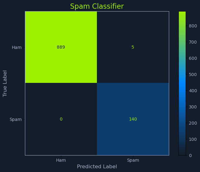
After training and fine-tuning the spam detection model, assessing its performance on new, unseen SMS messages is critical. This evaluation helps verify how well the model generalizes to real-world data and highlights improvement areas. The evaluation mirrors the preprocessing and feature extraction steps applied during training, ensuring a consistent and fair assessment of the model’s true predictive capabilities.
We begin by providing a list of new SMS messages for evaluation. These messages represent the types of inputs the model might receive in real-world use, including promotional offers, routine communications, urgent alerts, reminders, and incentive-based spam.
Code: python
# Example SMS messages for evaluation
new_messages = [
    "Congratulations! You've won a $1000 Walmart gift card. Go to http://bit.ly/1234 to claim now.",
    "Hey, are we still meeting up for lunch today?",
    "Urgent! Your account has been compromised. Verify your details here: www.fakebank.com/verify",
    "Reminder: Your appointment is scheduled for tomorrow at 10am.",
    "FREE entry in a weekly competition to win an iPad. Just text WIN to 80085 now!",
]
Before predicting with the trained model, we must preprocess the new messages using the same steps applied during training. Consistent preprocessing ensures that the model receives data in the same format it was trained on. The preprocess_message function converts each message to lowercase, removes non-alphabetic characters, tokenizes the text, removes stop words, and applies stemming.
Code: python
import numpy as np
import re

# Preprocess function that mirrors the training-time preprocessing
def preprocess_message(message):
    message = message.lower()
    message = re.sub(r"[^a-z\s$!]", "", message)
    tokens = word_tokenize(message)
    tokens = [word for word in tokens if word not in stop_words]
    tokens = [stemmer.stem(word) for word in tokens]
    return " ".join(tokens)
Next, we apply this function to each of the new messages:
Code: python
# Preprocess and vectorize messages
processed_messages = [preprocess_message(msg) for msg in new_messages]
The model expects numerical input features. To achieve this, we apply the same vectorization method used during training. The CountVectorizer saved within the pipeline (best_model.named_steps["vectorizer"]) transforms the preprocessed text into a numerical feature matrix.
Code: python
# Transform preprocessed messages into feature vectors
X_new = best_model.named_steps["vectorizer"].transform(processed_messages)
With the data properly preprocessed and vectorized, we feed the new messages into the trained MultinomialNB classifier (best_model.named_steps["classifier"]). This classifier outputs both a predicted label (spam or not spam) and class probabilities, indicating the model’s confidence in its decision.
Code: python
# Predict with the trained classifier
predictions = best_model.named_steps["classifier"].predict(X_new)
prediction_probabilities = best_model.named_steps["classifier"].predict_proba(X_new)
The next step is to present the evaluation results. For each message, we display:
Spam or Not-Spam).This output provides insight into the model’s reasoning and confidence levels, making it easier to understand and trust the predictions.
Code: python
# Display predictions and probabilities for each evaluated message
for i, msg in enumerate(new_messages):
    prediction = "Spam" if predictions[i] == 1 else "Not-Spam"
    spam_probability = prediction_probabilities[i][1]  # Probability of being spam
    ham_probability = prediction_probabilities[i][0]   # Probability of being not spam

    print(f"Message: {msg}")
    print(f"Prediction: {prediction}")
    print(f"Spam Probability: {spam_probability:.2f}")
    print(f"Not-Spam Probability: {ham_probability:.2f}")
    print("-" * 50)
A representative output might look like this:
Code: txt
Message: Congratulations! You've won a $1000 Walmart gift card. Go to http://bit.ly/1234 to claim now.
Prediction: Spam
Spam Probability: 1.00
Not-Spam Probability: 0.00
--------------------------------------------------
Message: Hey, are we still meeting up for lunch today?
Prediction: Not-Spam
Spam Probability: 0.00
Not-Spam Probability: 1.00
--------------------------------------------------
Message: Urgent! Your account has been compromised. Verify your details here: www.fakebank.com/verify
Prediction: Spam
Spam Probability: 0.94
Not-Spam Probability: 0.06
--------------------------------------------------
Message: Reminder: Your appointment is scheduled for tomorrow at 10am.
Prediction: Not-Spam
Spam Probability: 0.00
Not-Spam Probability: 1.00
--------------------------------------------------
Message: FREE entry in a weekly competition to win an iPad. Just text WIN to 80085 now!
Prediction: Spam
Spam Probability: 1.00
Not-Spam Probability: 0.00
--------------------------------------------------
These results show that the model can differentiate between benign messages and a range of spam content, providing both a categorical decision and the underlying probability estimates.
After confirming satisfactory performance, preserving the trained model to be reused later is often necessary. By saving the model to a file, users can avoid the computational expense of retraining it from scratch each time. This is especially helpful in production environments where quick predictions are required.
joblib is a Python library designed to efficiently serialize and deserialize Python objects, particularly those containing large arrays such as NumPy arrays or scikit-learn models. Serialization converts an in-memory object into a format that can be stored on disk or transmitted across networks. Deserialization involves converting the stored representation back into an in-memory object with the exact same state it had when saved.
joblib works by leveraging optimized binary file formats that compress and split objects, if necessary, to handle large datasets or complex models. When a model, such as a scikit-learn pipeline, is saved with joblib, it stores the entire model state including learned parameters and configurations. Later, when the model is reloaded, it will immediately be ready to make predictions as if it had just been trained.
By doing so, joblib helps streamline the deployment process. Instead of retraining the model every time the application restarts, developers and operations teams can load the saved model into memory and start making predictions. This reduces both computational overhead and startup latency.
Code: python
import joblib

# Save the trained model to a file for future use
model_filename = 'spam_detection_model.joblib'
joblib.dump(best_model, model_filename)

print(f"Model saved to {model_filename}")
In this example, best_model likely refers to a finalized and tested pipeline or classifier. The file spam_detection_model.joblib will contain all the necessary information to predict new data. To reuse the model later, load it back into the environment:
Code: python
loaded_model = joblib.load(model_filename)
predictions = loaded_model.predict(new_messages)
This approach ensures that the entire workflow—training, evaluating, and deploying the model—remains efficient and easily reproducible.
To evaluate your model, upload it to the evaluation portal running on the Playground VM. If you are not currently using the Playground VM, you can initialize it at the bottom of the page.
If you have the Playground VM running, you can use this Python script to upload your model from Jupyter directly. Once evaluated, if your model meets the required performance criteria, you will receive a flag value. This flag can be used to answer the question or verify the model’s success.
Code: python
import requests
import json

# Define the URL of the API endpoint
url = "http://localhost:8000/api/upload"

# Path to the model file you want to upload
model_file_path = "spam_detection_model.joblib"

# Open the file in binary mode and send the POST request
with open(model_file_path, "rb") as model_file:
    files = {"model": model_file}
    response = requests.post(url, files=files)

# Pretty print the response from the server
print(json.dumps(response.json(), indent=4))
If you are working from your own machine, ensure you have configured the HTB VPN to connect to the remote VM and spawned it. After connecting, access the model upload portal by navigating to http://<VM-IP>:8000/ in your browser and then uploading your model.
Anomaly detection identifies data points that deviate significantly from the norm. In cybersecurity, such anomalies can indicate malicious activities, network intrusions, or other security breaches. Random forests, which are ensembles of decision trees, effectively handle complex, high-dimensional data and can be used to detect these anomalous patterns.
A Random Forest is an ensemble machine-learning algorithm that builds multiple decision trees and aggregates their predictions. In classification tasks, each tree votes for a class, and the class receiving the majority votes is chosen. In regression tasks, the final prediction is the average of the individual tree outputs.
By combining the outputs of multiple trees, random forests often generalize better than a single decision tree, reducing overfitting and providing robust performance even in high-dimensional feature spaces.
Three key concepts shape the construction of a random forest:
Bootstrapping: Multiple subsets of the training data are created via sampling with replacement. Each subset trains a separate decision tree.Tree Construction: For each tree, a random subset of features is considered at every split, ensuring diversity and reducing correlations among trees.Voting: After all trees are trained, classification involves majority voting, while regression involves averaging predictions.When used for anomaly detection, a random forest is trained exclusively on data representing normal conditions. New, unseen data points are then evaluated against this learned normal behavior. Points that do not fit well, or that produce low confidence predictions, are flagged as potential anomalies.
This allows the model to detect unusual patterns, making it useful in scenarios such as identifying suspicious network traffic.
The NSL-KDD dataset refines the original KDD Cup 1999 dataset by eliminating redundant entries and correcting imbalanced class distributions. Researchers commonly adopt it as a standard reference for measuring the performance of various intrusion detection models.
NSL-KDD presents balanced, labeled instances of both normal and malicious network activities. This allows practitioners to perform not only binary classification (normal vs. abnormal) but also multi-class detection tasks targeting specific attack types. Such versatility makes NSL-KDD an invaluable resource for developing and testing intrusion detection techniques.
We'll be using a modified version of this dataset.
Before loading the NSL-KDD dataset, we must retrieve it from the provided URL. We can download the .zip file using Python's standard libraries and then extract it locally for further processing.
Code: python
import requests, zipfile, io

# URL for the NSL-KDD dataset
url = "https://academy.hackthebox.com/storage/modules/292/KDD_dataset.zip"

# Download the zip file and extract its contents
response = requests.get(url)
z = zipfile.ZipFile(io.BytesIO(response.content))
z.extractall('.')  # Extracts to the current directory
Properly loading the NSL-KDD dataset is essential before starting the preprocessing stage. This ensures that the data is consistently structured, with each column containing the correct information. Once loaded, the dataset can be inspected for quality, completeness, and potential preprocessing needs.
We begin by importing all necessary libraries.
Code: python
import numpy as np
import pandas as pd
from sklearn.ensemble import RandomForestClassifier
from sklearn.model_selection import train_test_split
from sklearn.metrics import accuracy_score, precision_score, recall_score, f1_score, confusion_matrix, classification_report
import seaborn as sns
import matplotlib.pyplot as plt
In this snippet:
numpy and pandas handle data loading and cleaning.RandomForestClassifier provides the algorithm we will use for anomaly detection.train_test_split and other metrics from sklearn.metrics support model evaluation and validation.seaborn and matplotlib assist in visualizing distributions, relationships, and model results.The NSL-KDD dataset includes a set of predefined features and labels. We must map these features to meaningful column names to work with them directly. We define a list of column names corresponding to the various observed characteristics of network connections and attacks. Additionally, we set file_path to point to the dataset file, ensuring that pandas know where to read the data from.
Code: python
# Set the file path to the dataset
file_path = r'KDD+.txt'

# Define the column names corresponding to the NSL-KDD dataset
columns = [
    'duration', 'protocol_type', 'service', 'flag', 'src_bytes', 'dst_bytes',
    'land', 'wrong_fragment', 'urgent', 'hot', 'num_failed_logins', 'logged_in',
    'num_compromised', 'root_shell', 'su_attempted', 'num_root', 'num_file_creations',
    'num_shells', 'num_access_files', 'num_outbound_cmds', 'is_host_login', 'is_guest_login',
    'count', 'srv_count', 'serror_rate', 'srv_serror_rate', 'rerror_rate', 'srv_rerror_rate',
    'same_srv_rate', 'diff_srv_rate', 'srv_diff_host_rate', 'dst_host_count', 'dst_host_srv_count',
    'dst_host_same_srv_rate', 'dst_host_diff_srv_rate', 'dst_host_same_src_port_rate',
    'dst_host_srv_diff_host_rate', 'dst_host_serror_rate', 'dst_host_srv_serror_rate',
    'dst_host_rerror_rate', 'dst_host_srv_rerror_rate', 'attack', 'level'
]
These column names ensure that each feature and label is properly identified. They include generic network statistics (e.g., duration, src_bytes, dst_bytes), categorical fields (protocol_type, service), and labels (attack, level), which classify the type of traffic observed.
With the file path and column names defined, we load the data into a pandas DataFrame. This provides a structured, tabular representation of the dataset, making it easier to inspect, preprocess, and visualize.
Code: python
# Read the combined NSL-KDD dataset into a DataFrame
df = pd.read_csv(file_path, names=columns)
By executing this code, we now have a DataFrame df containing all the data from the NSL-KDD dataset with the appropriate column headers. The DataFrame is ready for further inspection, cleaning, and preprocessing steps. Before proceeding, we can briefly examine the dataset’s structure, check for missing values, and confirm that all features align with their intended data types.
Code: python
print(df.head())
This section prepares the NSL-KDD dataset to train a random forest anomaly detection model. The primary goal is to transform the raw network traffic data into a usable format by creating classification targets, encoding categorical variables, and selecting important numeric features. We will produce both binary and multi-class targets, ensure that categorical data is machine-readable, and retain numeric metrics critical to the detection of abnormal traffic patterns.
The binary classification target identifies whether network traffic is normal or anomalous. We create a new column attack_flag in the DataFrame df to achieve this. Each row receives a label of 0 if the traffic is normal and 1 if it is an attack. This transformation simplifies the initial detection problem into a basic normal-versus-attack classification, which can be a starting point for a more granular analysis.
Code: python
# Binary classification target
# Maps normal traffic to 0 and any type of attack to 1
df['attack_flag'] = df['attack'].apply(lambda a: 0 if a == 'normal' else 1)
The value normal comes from the dataset; if we look at the dataset, you can see that all traffic is labeled normal or not:
Code: python
0,tcp,ftp_data,SF,491,0,0,0,0,0,0,0,0,0,0,0,0,0,0,0,0,0,2,2,0.0,0.0,0.0,0.0,1.0,0.0,0.0,150,25,0.17,0.03,0.17,0.0,0.0,0.0,0.05,0.0,normal,20
0,tcp,private,S0,0,0,0,0,0,0,0,0,0,0,0,0,0,0,0,0,0,0,123,6,1.0,1.0,0.0,0.0,0.05,0.07,0.0,255,26,0.1,0.05,0.0,0.0,1.0,1.0,0.0,0.0,neptune,19
While a binary target is useful, it lacks granularity. To address this, we also create a multi-class classification target that distinguishes between different categories of attacks. We define lists categorizing specific attacks into four major groups:
DoS (Denial of Service) attacks such as neptune and smurfProbe attacks that scan networks for vulnerabilities, like satan or ipsweepPrivilege Escalation attacks that attempt to gain unauthorized admin-level control, such as buffer_overflowAccess attacks that seek to breach system access controls, like guess_passwdA custom function map_attack checks the type of attack and assigns it an integer:
0 for normal traffic1 for DoS attacks2 for Probe attacks3 for Privilege Escalation attacks4 for Access attacksThis expanded classification target allows models to learn to distinguish between normal and abnormal traffic and the nature of the observed attacks.
Code: python
# Multi-class classification target categories
dos_attacks = ['apache2', 'back', 'land', 'neptune', 'mailbomb', 'pod',
               'processtable', 'smurf', 'teardrop', 'udpstorm', 'worm']
probe_attacks = ['ipsweep', 'mscan', 'nmap', 'portsweep', 'saint', 'satan']
privilege_attacks = ['buffer_overflow', 'loadmdoule', 'perl', 'ps',
                     'rootkit', 'sqlattack', 'xterm']
access_attacks = ['ftp_write', 'guess_passwd', 'http_tunnel', 'imap',
                  'multihop', 'named', 'phf', 'sendmail', 'snmpgetattack',
                  'snmpguess', 'spy', 'warezclient', 'warezmaster',
                  'xclock', 'xsnoop']

def map_attack(attack):
    if attack in dos_attacks:
        return 1
    elif attack in probe_attacks:
        return 2
    elif attack in privilege_attacks:
        return 3
    elif attack in access_attacks:
        return 4
    else:
        return 0

# Assign multi-class category to each row
df['attack_map'] = df['attack'].apply(map_attack)
Network traffic data often includes categorical attributes that are not directly usable by machine learning algorithms, which generally require numeric inputs. Two important features in the NSL-KDD dataset are protocol_type (e.g., tcp, udp) and service (e.g., http, ftp). These features categorize the nature of network interactions but must be transformed into numeric form.
We use one-hot encoding, provided by the get_dummies function in pandas. This approach creates a binary indicator variable for each category, ensuring that no ordinal relationship is implied between different protocols or services. After encoding, each categorical value is represented by a separate column indicating its presence (1) or absence (0).
Code: python
# Encoding categorical variables
features_to_encode = ['protocol_type', 'service']
encoded = pd.get_dummies(df[features_to_encode])
Beyond categorical variables, the dataset contains a range of numeric features that describe various aspects of network traffic. These include basic metrics like duration, src_bytes, and dst_bytes, as well as more specialized features such as serror_rate and dst_host_srv_diff_host_rate, which capture statistical properties of the network sessions. By selecting these numeric features, we ensure the model has access to both raw volume data and more nuanced, derived statistics that help distinguish normal from abnormal patterns.
Code: python
# Numeric features that capture various statistical properties of the traffic
numeric_features = [
    'duration', 'src_bytes', 'dst_bytes', 'wrong_fragment', 'urgent', 'hot',
    'num_failed_logins', 'num_compromised', 'root_shell', 'su_attempted',
    'num_root', 'num_file_creations', 'num_shells', 'num_access_files',
    'num_outbound_cmds', 'count', 'srv_count', 'serror_rate',
    'srv_serror_rate', 'rerror_rate', 'srv_rerror_rate', 'same_srv_rate',
    'diff_srv_rate', 'srv_diff_host_rate', 'dst_host_count', 'dst_host_srv_count',
    'dst_host_same_srv_rate', 'dst_host_diff_srv_rate',
    'dst_host_same_src_port_rate', 'dst_host_srv_diff_host_rate',
    'dst_host_serror_rate', 'dst_host_srv_serror_rate', 'dst_host_rerror_rate',
    'dst_host_srv_rerror_rate'
]
The final step is to combine the one-hot encoded categorical features with the selected numeric features. We join them into a single DataFrame train_set that will serve as the primary input to our machine-learning model. We also store the multi-class target variable attack_map as multi_y for classification tasks. At this stage, the data is in a suitable format for splitting into training, validation, test sets, and subsequently training the random forest anomaly detection model.
Code: python
# Combine encoded categorical variables and numeric features
train_set = encoded.join(df[numeric_features])

# Multi-class target variable
multi_y = df['attack_map']
In the Data Transformation section, we discussed the rationale and methods for splitting data into training, validation, and test sets. We now apply those principles specifically to the NSL-KDD dataset, ensuring that our random forest anomaly detection model is trained, tuned, and evaluated on distinct subsets.
We use train_test_split to allocate a portion of the data for testing, ensuring that our final evaluations occur on unseen data.
Code: python
# Split data into training and test sets for multi-class classification
train_X, test_X, train_y, test_y = train_test_split(train_set, multi_y, test_size=0.2, random_state=1337)
We further split the training data to create a validation set. This supports model tuning and hyperparameter optimization without contaminating the final test data.
Code: python
# Further split the training set into separate training and validation sets
multi_train_X, multi_val_X, multi_train_y, multi_val_y = train_test_split(train_X, train_y, test_size=0.3, random_state=1337)
After splitting, we have:
train_X, train_y: Core training settest_X, test_y: Reserved for the final performance evaluationmulti_train_X, multi_train_y: Training subset for fitting the modelmulti_val_X, multi_val_y: Validation subset for hyperparameter tuningThis careful partitioning, applied after the transformations and encodings discussed earlier, ensures that the model development process remains consistent and that the final evaluation is unbiased and reflective of real-world performance.
In this section, we will train a random forest model on the NSL-KDD dataset for multi-class classification. The goal is to build a model that can accurately classify network traffic into different attack categories or as normal traffic.
Code: python
# Train RandomForest model for multi-class classification
rf_model_multi = RandomForestClassifier(random_state=1337)
rf_model_multi.fit(multi_train_X, multi_train_y)
The first step in this process is to train the random forest model using the training subset of the dataset. We initialize a RandomForestClassifier with the random_state parameter set to 1337 to ensure reproducibility. The fit method is then used to train the model on the features multi_train_X and the target variable multi_train_y. This step builds the model by learning patterns from the training data.
Next, we will evaluate the performance of the trained random forest model on the validation set. The goal is to assess the model's accuracy and other performance metrics to ensure it generalizes well to unseen data.
Code: python
# Predict and evaluate the model on the validation set
multi_predictions = rf_model_multi.predict(multi_val_X)
accuracy = accuracy_score(multi_val_y, multi_predictions)
precision = precision_score(multi_val_y, multi_predictions, average='weighted')
recall = recall_score(multi_val_y, multi_predictions, average='weighted')
f1 = f1_score(multi_val_y, multi_predictions, average='weighted')
print(f"Validation Set Evaluation:")
print(f"Accuracy: {accuracy:.4f}")
print(f"Precision: {precision:.4f}")
print(f"Recall: {recall:.4f}")
print(f"F1-Score: {f1:.4f}")

# Confusion Matrix for Validation Set
conf_matrix = confusion_matrix(multi_val_y, multi_predictions)
class_labels = ['Normal', 'DoS', 'Probe', 'Privilege', 'Access']
sns.heatmap(conf_matrix, annot=True, fmt='d', cmap='Blues',
            xticklabels=class_labels,
            yticklabels=class_labels)
plt.title('Network Anomaly Detection - Validation Set')
plt.xlabel('Predicted')
plt.ylabel('Actual')
plt.show()

# Classification Report for Validation Set
print("Classification Report for Validation Set:")
print(classification_report(multi_val_y, multi_predictions, target_names=class_labels))
After training the model, we use it to make predictions on the validation set. The predict method of the RandomForestClassifier is used to generate predictions for the features multi_val_X. We then calculate various performance metrics using functions from sklearn.metrics:
Accuracy: The proportion of correctly classified instances.Precision: The ratio of true positive predictions to the total predicted positives.Recall: The ratio of true positive predictions to the total actual positives.F1-Score: The harmonic mean of precision and recall.These metrics are printed to evaluate the model's performance on the validation set comprehensively.
We also generate a confusion matrix using confusion_matrix and visualize it using seaborn and matplotlib. The confusion matrix provides a detailed breakdown of the model's predictions, showing each class's number of true positives, true negatives, false positives, and false negatives.
Finally, we print a classification report that includes precision, recall, F1-score, and support for each class. This report gives a more granular view of the model's performance across different classes.
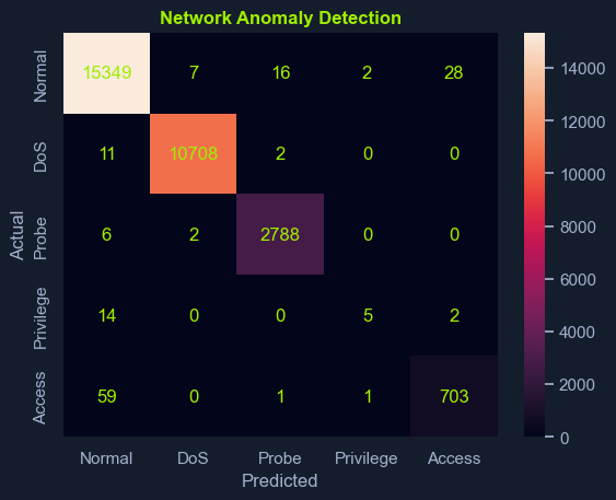
Next, we will evaluate the final performance of the trained random forest model on the test set. The goal is to assess the model's ability to generalize to completely unseen data and provide a final evaluation of its performance.
Code: python
# Final evaluation on the test set
test_multi_predictions = rf_model_multi.predict(test_X)
test_accuracy = accuracy_score(test_y, test_multi_predictions)
test_precision = precision_score(test_y, test_multi_predictions, average='weighted')
test_recall = recall_score(test_y, test_multi_predictions, average='weighted')
test_f1 = f1_score(test_y, test_multi_predictions, average='weighted')
print("\nTest Set Evaluation:")
print(f"Accuracy: {test_accuracy:.4f}")
print(f"Precision: {test_precision:.4f}")
print(f"Recall: {test_recall:.4f}")
print(f"F1-Score: {test_f1:.4f}")

# Confusion Matrix for Test Set
test_conf_matrix = confusion_matrix(test_y, test_multi_predictions)
sns.heatmap(test_conf_matrix, annot=True, fmt='d', cmap='Blues',
            xticklabels=class_labels,
            yticklabels=class_labels)
plt.title('Network Anomaly Detection')
plt.xlabel('Predicted')
plt.ylabel('Actual')
plt.show()

# Classification Report for Test Set
print("Classification Report for Test Set:")
print(classification_report(test_y, test_multi_predictions, target_names=class_labels))
The final step in our process is to evaluate the model on the test set. We use the predict method to generate predictions for the features test_X. Similar to the validation set evaluation, we calculate and print various performance metrics:
Accuracy: The proportion of correctly classified instances.Precision: The ratio of true positive predictions to the total predicted positives.Recall: The ratio of true positive predictions to the total actual positives.F1-Score: The harmonic mean of precision and recall.We also generate a confusion matrix for the test set and visualize it using seaborn and matplotlib. This matrix provides a detailed breakdown of the model's predictions on the test data, showing each class's number of true positives, true negatives, false positives, and false negatives.
Finally, we print a classification report that includes precision, recall, F1-score, and support for each class. This report gives a comprehensive view of the model's performance across different classes on the test set.
By executing this code, we have trained a random forest model, evaluated its performance on both the validation and test sets, and generated detailed reports and visualizations to assess its effectiveness in classifying network traffic.
Save your model using this code:
Code: python
import joblib

# Save the trained model to a file
model_filename = 'network_anomaly_detection_model.joblib'
joblib.dump(rf_model_multi, model_filename)

print(f"Model saved to {model_filename}")
To evaluate your model, upload it to the evaluation portal running on the Playground VM. If you are not currently using the Playground VM, you can initialize it at the bottom of the page.
If you have the Playground VM running, you can use this Python script to upload your model from Jupyter directly. Once evaluated, if your model meets the required performance criteria, you will receive a flag value. This flag can be used to answer the question or verify the model’s success.
Code: python
import requests
import json

# Define the URL of the API endpoint
url = "http://localhost:8001/api/upload"

# Path to the model file you want to upload
model_file_path = "network_anomaly_detection_model.joblib"

# Open the file in binary mode and send the POST request
with open(model_file_path, "rb") as model_file:
    files = {"model": model_file}
    response = requests.post(url, files=files)

# Pretty print the response from the server
print(json.dumps(response.json(), indent=4))
If you are working from your own machine, ensure you have configured the HTB VPN to connect to the remote VM and spawned it. After connecting, access the model upload portal by navigating to http://<VM-IP>:8001/ in your browser and then uploading your model.
Malware is software designed to cause damage or unauthorized actions on a computer system or network. Malware can be categorized based on its characteristics, mode of operation, and purpose, among other factors. A malware category is commonly referred to as a malware family. We can look at malpedia to explore details about different malware families. Famous examples include Emotet and WannaCry.
Features of malware to consider for classification include its behavior or functionality, delivery and propagation methods, and technical traits. As such, manual malware classification requires a combination of static and dynamic analysis, including time-consuming reverse engineering of the malware binary. Thus, using ML classifiers to aid in malware classification can significantly speed up the process.
In this section, we will implement a malware classifier based on the technique explored in this paper, which explores malware classification based on malware images.
While classifying malware based on images might initially sound counterintuitive, we will explore the dataset in the upcoming section and learn why this approach makes sense. For this module, training a classifier on images has the obvious advantage that we do not have to handle potentially dangerous malicious binaries directly. By only handling images that represent these binaries, we cannot accidentally infect our system with malware. Therefore, it is more appropriate for a learning environment than dealing with the binary files directly.
In the upcoming sections, we will explore the process of training a CNN to classify the malware images.
The dataset of malware images we will be using is the malimg dataset, which we can obtain here or here. It was proposed in this paper.
We can download and unpack the dataset using the following commands:
The Malware Dataset
root@htb[/htb]$ wget https://www.kaggle.com/api/v1/datasets/download/ikrambenabd/malimg-original -O malimg.zip

root@htb[/htb]$ unzip malimg.zip
The dataset consists of 9339 image files for 25 different malware families. The dataset is organized in folders, where each folder contains all samples for a single malware family. The folder name corresponds to the malware family's name:
The Malware Dataset
root@htb[/htb]$ ls malimg_paper_dataset_imgs

 Adialer.C        C2LOP.P          Lolyda.AA3      'Swizzor.gen!I'
 Agent.FYI        Dialplatform.B   Lolyda.AT        VB.AT
 Allaple.A        Dontovo.A       'Malex.gen!J'     Wintrim.BX
 Allaple.L        Fakerean         Obfuscator.AD    Yuner.A
'Alueron.gen!J'   Instantaccess   'Rbot!gen'
 Autorun.K        Lolyda.AA1       Skintrim.N
'C2LOP.gen!g'     Lolyda.AA2      'Swizzor.gen!E'
Each image contains a visual representation of a PE file, which is a Windows executable. The images are grayscale in png format:

These images are a direct representation of the malware binaries. Each pixel in the image represents a single byte in the binary. The byte can be any value in the 0-255 range. The exact value is represented in the corresponding pixel's brightness. A byte with the value 0 results in a black pixel, a value of 255 results in a white pixel, and a value in between results in the corresponding gray pixel.
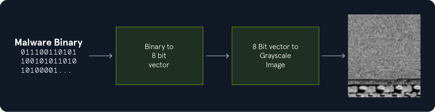
Each binary byte is fully encoded within the image, meaning the image can be used to exactly reconstruct the binary without any loss of information. Furthermore, the images can visibly convey patterns in the binary. For instance, consider the following two image samples from the FakeRean malware family. We can see distinct patterns in both malware images.


To familiarize ourselves with the dataset, let's start exploring it by creating a plot of the class distribution within it. This enables us to spot classes that are over- or underrepresented.
To achieve this, we will need the following imports as well as a base path to the folder containing the data:
Code: python
import os
import matplotlib.pyplot as plt
import seaborn as sns

DATA_BASE_PATH = "./malimg_paper_dataset_imgs/"
Afterward, we can iterate over all malware families and count the number of images within the corresponding folder to compute the overall class distribution:
Code: python
# compute the class distribution
dist = {}
for mlw_class in os.listdir(DATA_BASE_PATH):
    mlw_dir = os.path.join(DATA_BASE_PATH, mlw_class)
    dist[mlw_class] = len(os.listdir(mlw_dir))
Finally, we can create a barplot to visualize the class distribution:
Code: python
# plot the class distribution

# HTB Color Palette
htb_green = "#9FEF00"
node_black = "#141D2B"
hacker_grey = "#A4B1CD"

# data
classes = list(dist.keys())
frequencies = list(dist.values())

# plot
plt.figure(facecolor=node_black)
sns.barplot(y=classes, x=frequencies, edgecolor = "black", orient='h', color=htb_green)
plt.title("Malware Class Distribution", color=htb_green)
plt.xlabel("Malware Class Frequency", color=htb_green)
plt.ylabel("Malware Class", color=htb_green)
plt.xticks(color=hacker_grey)
plt.yticks(color=hacker_grey)
ax = plt.gca()
ax.set_facecolor(node_black)
ax.spines['bottom'].set_color(hacker_grey)
ax.spines['top'].set_color(node_black)
ax.spines['right'].set_color(node_black)
ax.spines['left'].set_color(hacker_grey)
plt.show()
From the resulting diagram, we can identify which malware families are represented more than others, potentially skewing the model. Suppose the trained model does not provide the expected performance in accuracy, number of false positives, and number of false negatives. In that case, we may want to fine-tune the dataset before training to ensure a more balanced class distribution.
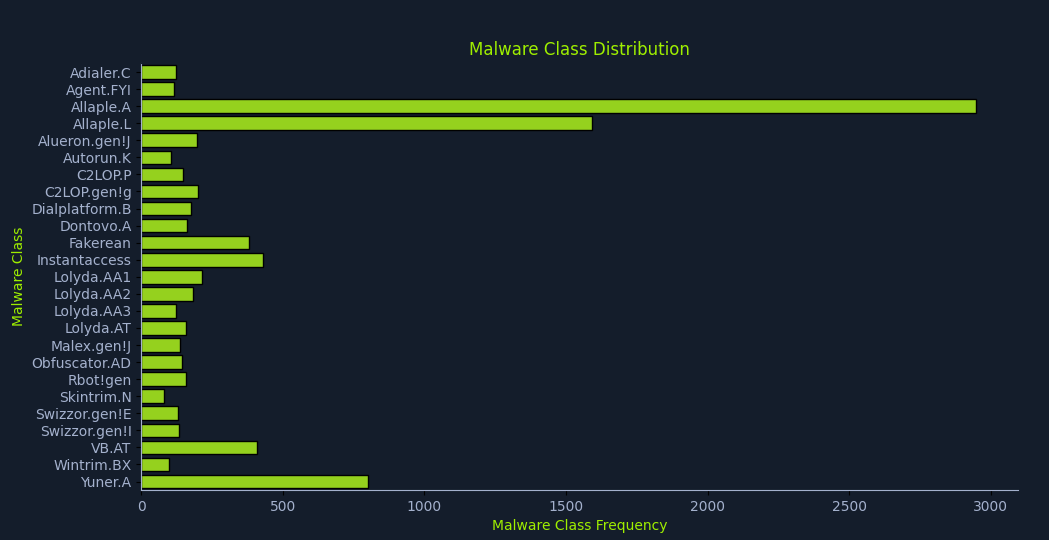
We need to prepare the data before we can feed the images to a CNN for training and inference. In particular, we need to split the data into two distinct datasets: a training and a test set. Furthermore, we need to apply the preprocessing functions expected by our model so the model can work on the images. Lastly, we must create DataLoaders that we can use during training and inference.
To split the data into two distinct datasets, one for training and one for testing, we will use the library split-folders, which we can install with pip:
Preprocessing the Malware Dataset
root@htb[/htb]$ pip3 install split-folders
Afterward, we can use the following code to split the data accordingly. We will use an 80-20 split, meaning 80% of the data will be used for training and 20% for testing:
Code: python
import splitfolders

DATA_BASE_PATH = "./malimg_paper_dataset_imgs/"
TARGET_BASE_PATH = "./newdata/"

TRAINING_RATIO = 0.8
TEST_RATIO = 1 - TRAINING_RATIO

splitfolders.ratio(input=DATA_BASE_PATH, output=TARGET_BASE_PATH, ratio=(TRAINING_RATIO, 0, TEST_RATIO))
After running the code once, a new directory ./newdata/ will be created containing three folders:
Preprocessing the Malware Dataset
root@htb[/htb]$ ls -la ./newdata/

total 0
drwxr-xr-x 1 t t  24 26. Nov 10:52 .
drwxr-xr-x 1 t t 160 26. Nov 10:52 ..
drwxr-xr-x 1 t t 498 26. Nov 10:52 test
drwxr-xr-x 1 t t 498 26. Nov 10:52 train
drwxr-xr-x 1 t t 498 26. Nov 10:52 val
The test folder contains the test dataset, the train folder contains the training dataset, and the val folder contains the validation dataset. In this case, we will not use a validation data set, which is why the validation data set is empty. We can confirm the 80-20 split by counting the number of files in each dataset:
Preprocessing the Malware Dataset
root@htb[/htb]$ find ./newdata/test/ -type f | wc -l

1880
Preprocessing the Malware Dataset
root@htb[/htb]$ find ./newdata/train/ -type f | wc -l

7459
Preprocessing the Malware Dataset
root@htb[/htb]$ find ./newdata/val/ -type f | wc -l

0
The split was successful, as we can see. We can now create DataLoaders for training and inference and apply the required preprocessing to the images.
In the first step, let us define the preprocessing required for our model to read the data. For CNNs, this typically requires a resizing such that all input images are the same size and a normalization. Normalization ensures that the data is standardized before the data is fed to the model. This results in a model that is easier to train. In PyTorch, our preprocessing looks like this:
Code: python
from torchvision import transforms

# Define preprocessing transforms
transform = transforms.Compose([
    transforms.Resize((75, 75)),
    transforms.ToTensor(),
    transforms.Normalize(mean=[0.485, 0.456, 0.406], std=[0.229, 0.224, 0.225])
])
Afterward, we can load the datasets from their corresponding folders and apply the preprocessing functions. We need to specify the root folder for each dataset in the root parameter and the preprocessing transform in the transform parameter. As we have discussed above, the root folders for the datasets are ./newdata/train/ and ./newdata/test/, respectively.
Code: python
from torchvision.datasets import ImageFolder
import os

BASE_PATH = "./newdata/"

# Load training and test datasets
train_dataset = ImageFolder(
    root=os.path.join(BASE_PATH, "train"),
    transform=transform
)

test_dataset = ImageFolder(
    root=os.path.join(BASE_PATH, "test"),
    transform=transform
)
Finally, we can create DataLoader instances, which we can use to iterate over the data for training and inference. We can supply a batch size and specify the number of workers to load the data in the num_workers parameter. This enables parallelization and will speed up the data handling:
Code: python
from torch.utils.data import DataLoader

TRAIN_BATCH_SIZE = 1024
TEST_BATCH_SIZE = 1024

# Create data loaders
train_loader = DataLoader(
    train_dataset,
    batch_size=TRAIN_BATCH_SIZE,
    shuffle=True,
    num_workers=2
)

test_loader = DataLoader(
    test_dataset,
    batch_size=TEST_BATCH_SIZE,
    shuffle=False,
    num_workers=2
)
Let us take a look at one of the preprocessed images to see its effects:
Code: python
import matplotlib.pyplot as plt

# HTB Color Palette
htb_green = "#9FEF00"
node_black = "#141D2B"
hacker_grey = "#A4B1CD"

# image
sample = next(iter(train_loader))[0][0]

# plot
plt.figure(facecolor=node_black)
plt.imshow(sample.permute(1,2,0))
plt.xticks(color=hacker_grey)
plt.yticks(color=hacker_grey)
ax = plt.gca()
ax.set_facecolor(node_black)
ax.spines['bottom'].set_color(hacker_grey)
ax.spines['top'].set_color(node_black)
ax.spines['right'].set_color(node_black)
ax.spines['left'].set_color(hacker_grey)
ax.tick_params(axis='x', colors=hacker_grey)
ax.tick_params(axis='y', colors=hacker_grey)
plt.show()
This is the raw malware image:

This is the resized and normalized image from our DataLoader that we will feed to the model:
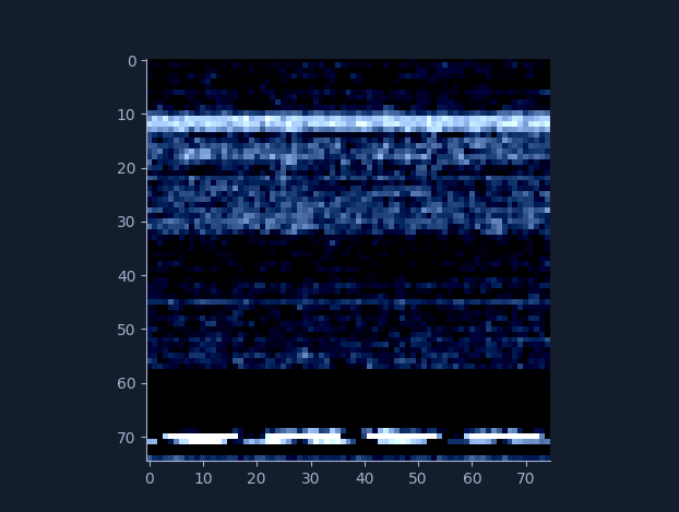
The details can be roughly discerned from the raw image. However, many of the fine details have been lost.
After combining the above code into a single function, we end up with the following code:
Code: python
from torchvision import transforms
from torch.utils.data import DataLoader
from torchvision.datasets import ImageFolder
import os

def load_datasets(base_path, train_batch_size, test_batch_size):
    # Define preprocessing transforms
    transform = transforms.Compose([
        transforms.Resize((75, 75)),
        transforms.ToTensor(),
        transforms.Normalize(mean=[0.485, 0.456, 0.406], std=[0.229, 0.224, 0.225])
    ])

    # Load training and test datasets
    train_dataset = ImageFolder(
        root=os.path.join(base_path, "train"),
        transform=transform
    )

    test_dataset = ImageFolder(
        root=os.path.join(base_path, "test"),
        transform=transform
    )

    # Create data loaders
    train_loader = DataLoader(
        train_dataset,
        batch_size=train_batch_size,
        shuffle=True,
        num_workers=2
    )

    test_loader = DataLoader(
        test_dataset,
        batch_size=test_batch_size,
        shuffle=False,
        num_workers=2
    )

    n_classes = len(train_dataset.classes)
    return train_loader, test_loader, n_classes
Note that the function also returns the number of classes in the dataset. As we have mentioned before, the Malimg dataset consists of 25 classes, so we could omit this step and simply assume there are always 25 classes. However, by reading this information dynamically from the data itself, we can use the same code even after making changes to the dataset, either by removing one of the classes or adding new classes to the dataset.
The heart of any classifier is the model. As discussed previously, we will be using a CNN model. To speed up the training process, we will base our model on a pre-trained version of a well-established CNN called ResNet50.
The ResNet family of CNNs was proposed in 2015 in this paper. We will use a variant called ResNet50. This model is 50 layers deep, where it got its name, and consists of roughly 23 million parameters. This model is strong in image classification tasks, which perfectly fits our needs for malware classification.
To significantly speed up the training process, we will not start with randomly initialized weights but rather with a pre-trained ResNet50 model. Our code will download pre-trained weights and apply them to our model as a baseline. We will then run our training on the malware image dataset to fine-tune it for our purpose. This approach will save us training time in the magnitude of multiple days or even weeks.
Furthermore, to further speed up the training process, we will freeze the weights of all ResNet layers except for the final one. Thus, during our training process, only the weights of the final layer will change. While this may reduce our classifier's performance, it will significantly benefit our training time and be a good trade-off for our simple proof-of-concept experiment. We will also adjust the final layer according to our needs. In particular, we may adjust the number of neurons in the final layer and fix the output size to the number of classes in our training data. This results in the following MalwareClassifier class:
Code: python
import torch.nn as nn
import torchvision.models as models

HIDDEN_LAYER_SIZE = 1000

class MalwareClassifier(nn.Module):
    def __init__(self, n_classes):
        super(MalwareClassifier, self).__init__()
        # Load pretrained ResNet50
        self.resnet = models.resnet50(weights='DEFAULT')

        # Freeze ResNet parameters
        for param in self.resnet.parameters():
            param.requires_grad = False

        # Replace the last fully connected layer
        num_features = self.resnet.fc.in_features
        self.resnet.fc = nn.Sequential(
            nn.Linear(num_features, HIDDEN_LAYER_SIZE),
            nn.ReLU(),
            nn.Linear(HIDDEN_LAYER_SIZE, n_classes)
        )

    def forward(self, x):
        return self.resnet(x)
When initializing the model, we need to specify the number of classes. Since our dataset consists of 25 classes, we can initialize the model like so:
Code: python
model = MalwareClassifier(25)
However, as discussed in the previous section, the advantage of dynamically setting the number of classes is that we can directly use it from the dataset. By combining the above code with the code from the previous section, we can take the number of classes from the dataset and initialize the model accordingly:
Code: python
DATA_PATH = "./newdata/"
TRAINING_BATCH_SIZE = 1024
TEST_BATCH_SIZE = 1024

# Load datasets
train_loader, test_loader, n_classes = load_datasets(DATA_PATH, TRAINING_BATCH_SIZE, TEST_BATCH_SIZE)

# Initialize model
model = MalwareClassifier(n_classes)
After loading the datasets and initializing the model, let's finally discuss model training and evaluation to see how well our model performs.
Let us define a training function that takes a model, a training loader, and the number of epochs. We will then specify the loss function as CrossEntropyLoss and use the Adam optimizer. Afterward, we iterate the entire training data for each epoch and run the forward and backward passes. For a refresher on backpropagation and gradient descent, check out the Fundamentals of AI module.
The final training function looks like this:
Code: python
import torch
import time

def train(model, train_loader, n_epochs, verbose=False):
    model.train()
    criterion = torch.nn.CrossEntropyLoss()
    optimizer = torch.optim.Adam(model.parameters())

    training_data = {"accuracy": [], "loss": []}

    for epoch in range(n_epochs):
        running_loss = 0
        n_total = 0
        n_correct = 0
        checkpoint = time.time() * 1000

        for inputs, labels in train_loader:
            optimizer.zero_grad()
            outputs = model(inputs)
            loss = criterion(outputs, labels)
            loss.backward()
            optimizer.step()

            _, predicted = outputs.max(1)
            n_total += labels.size(0)
            n_correct += predicted.eq(labels).sum().item()
            running_loss += loss.item()

        epoch_loss = running_loss / len(train_loader)
        epoch_duration = int(time.time() * 1000 - checkpoint)
        epoch_accuracy = compute_accuracy(n_correct, n_total)

        training_data["accuracy"].append(epoch_accuracy)
        training_data["loss"].append(epoch_loss)

        if verbose:
            print(f"[i] Epoch {epoch+1} of {n_epochs}: Acc: {epoch_accuracy:.2f}% Loss: {epoch_loss:.4f} (Took {epoch_duration} ms).")

    return training_data
Note that much of the code within the training function keeps track of information about the training, such as time elapsed, accuracy, and loss.
Additionally, we will define a function to save the trained model to disk for later use:
Code: python
def save_model(model, path):
    model_scripted = torch.jit.script(model)
    model_scripted.save(path)
To evaluate the model, we will first define a function that runs the model on a single input and returns the predicted class:
Code: python
def predict(model, test_data):
    model.eval()

    with torch.no_grad():
        output = model(test_data)
        _, predicted = torch.max(output.data, 1)

    return predicted
We set the model to evaluation mode using the call model.eval() and disable gradient calculation using torch.no_grad(). From there, we can write an evaluation function that iterates over the entire test dataset and evaluates the model's performance in terms of accuracy:
Code: python
def compute_accuracy(n_correct, n_total):
    return round(100 * n_correct / n_total, 2)


def evaluate(model, test_loader):
    model.eval()

    n_correct = 0
    n_total = 0

    with torch.no_grad():
        for data, target in test_loader:
            predicted = predict(model, data)
            n_total += target.size(0)
            n_correct += (predicted == target).sum().item()

    accuracy = compute_accuracy(n_correct, n_total)

    return accuracy
Lastly, let us define a couple of helper functions that create simple plots for the training accuracy and loss per epoch, respectively:
Code: python
import matplotlib.pyplot as plt

def plot(data, title, label, xlabel, ylabel):
    # HTB Color Palette
    htb_green = "#9FEF00"
    node_black = "#141D2B"
    hacker_grey = "#A4B1CD"

    # plot
    plt.figure(figsize=(10, 6), facecolor=node_black)
    plt.plot(range(1, len(data)+1), data, label=label, color=htb_green)
    plt.title(title, color=htb_green)
    plt.xlabel(xlabel, color=htb_green)
    plt.ylabel(ylabel, color=htb_green)
    plt.xticks(color=hacker_grey)
    plt.yticks(color=hacker_grey)
    ax = plt.gca()
    ax.set_facecolor(node_black)
    ax.spines['bottom'].set_color(hacker_grey)
    ax.spines['top'].set_color(node_black)
    ax.spines['right'].set_color(node_black)
    ax.spines['left'].set_color(hacker_grey)

    legend = plt.legend(facecolor=node_black, edgecolor=hacker_grey, fontsize=10)
    plt.setp(legend.get_texts(), color=htb_green)

    plt.show()

def plot_training_accuracy(training_data):
    plot(training_data['accuracy'], "Training Accuracy", "Accuracy", "Epoch", "Accuracy (%)")

def plot_training_loss(training_data):
    plot(training_data['loss'], "Training Loss", "Loss", "Epoch", "Loss")
After defining all helper functions, we can write a script that defines all parameters and runs the helper functions to load the data, initialize the model, train the model, save the model, and finally evaluate the model:
Code: python
# data parameters
DATA_PATH = "./newdata/"

# training parameters
N_EPOCHS = 10
TRAINING_BATCH_SIZE = 512
TEST_BATCH_SIZE = 1024

# model parameters
HIDDEN_LAYER_SIZE = 1000
MODEL_FILE = "malware_classifier.pth"


# Load datasets
train_loader, test_loader, n_classes = load_datasets(DATA_PATH, TRAINING_BATCH_SIZE, TEST_BATCH_SIZE)

# Initialize model
model = MalwareClassifier(n_classes)

# Train model
print("[i] Starting Training...")
training_information = train(model, train_loader, N_EPOCHS, verbose=True)

# Save model
save_model(model, MODEL_FILE)

# evaluate model
accuracy = evaluate(model, test_loader)
print(f"[i] Inference accuracy: {accuracy}%.")

# Plot training details
plot_training_accuracy(training_information)
plot_training_loss(training_information)
Running the final code, we can achieve an accuracy of 88.54% on the test dataset:
Training and Evaluation (Malware Image Classification)
root@htb[/htb]$ python3 main.py

[i] Epoch 1 of 10: Acc: 57.09% Loss: 1.4741 (Took 41128 ms).
[i] Epoch 2 of 10: Acc: 85.01% Loss: 0.4631 (Took 40630 ms).
[i] Epoch 3 of 10: Acc: 89.60% Loss: 0.2880 (Took 39567 ms).
[i] Epoch 4 of 10: Acc: 91.88% Loss: 0.2294 (Took 39464 ms).
[i] Epoch 5 of 10: Acc: 92.97% Loss: 0.2113 (Took 39367 ms).
[i] Epoch 6 of 10: Acc: 93.86% Loss: 0.1744 (Took 39172 ms).
[i] Epoch 7 of 10: Acc: 95.13% Loss: 0.1572 (Took 39804 ms).
[i] Epoch 8 of 10: Acc: 94.81% Loss: 0.1501 (Took 39092 ms).
[i] Epoch 9 of 10: Acc: 96.51% Loss: 0.1188 (Took 39328 ms).
[i] Epoch 10 of 10: Acc: 96.26% Loss: 0.1198 (Took 39125 ms).
[i] Inference accuracy: 88.54%.
During the training process, we can observe a steady increase in accuracy up until the final couple of epochs:
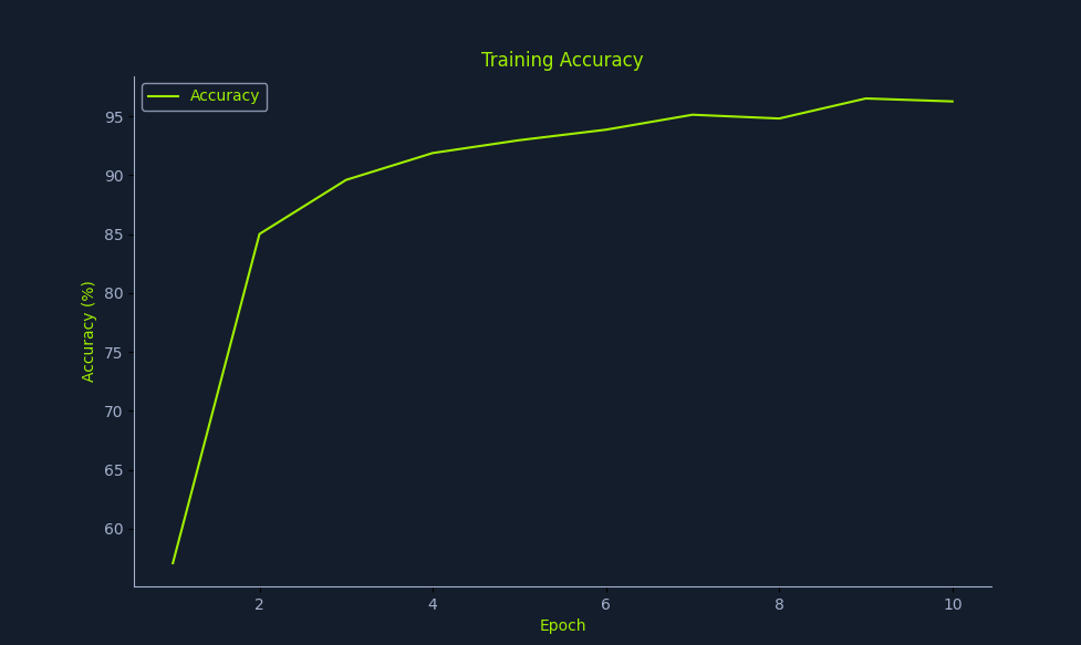
While the final accuracy is not great, it is acceptable, provided our simple training setup. We have tweaked many parameters to favor training time instead of model performance. Keep in mind that the model's accuracy may vary depending on the random split of the datasets. Additionally, tweaking the parameters affects both training time and model performance. Feel free to play around with all the parameters the script defines to determine their effects.
To evaluate your model, upload it to the evaluation portal running on the Playground VM. If you are not currently using the Playground VM, you can initialize it at the bottom of the page.
If you have the Playground VM running, you can use this Python script to upload your model from Jupyter directly. Once evaluated, if your model meets the required performance criteria, you will receive a flag value. This flag can be used to answer the question or verify the model’s success.
Code: python
import requests
import json

# Define the URL of the API endpoint
url = "http://localhost:8002/api/upload"

# Path to the model file you want to upload
model_file_path = "malware_classifier.pth"

# Open the file in binary mode and send the POST request
with open(model_file_path, "rb") as model_file:
    files = {"model": model_file}
    response = requests.post(url, files=files)

# Pretty print the response from the server
print(json.dumps(response.json(), indent=4))
If you are working from your own machine, ensure you have configured the HTB VPN to connect to the remote VM, and you have spawned it. After connecting, access the model upload portal by navigating to http://<VM-IP>:8002/ in your browser, and then upload your model.
Note: Training time for a single epoch in the Playground environment may take up to 10 minutes. Three epochs should be sufficient to reach the required accuracy. Evaluating an uploaded model may take up to two minutes. Training time on your own system should be much faster, depending on your hardware.
The IMDB dataset introduced by Maas et al. (2011) provides a collection of movie reviews extracted from the Internet Movie Database, annotated for sentiment analysis. It includes 50,000 reviews split evenly into training and test sets, and its carefully curated mixture of positive and negative examples allows researchers to benchmark and improve various natural language processing techniques. The IMDB dataset has influenced subsequent work in developing vector-based word representations and remains a popular baseline resource for evaluating classification performance and model architectures in sentiment classification tasks (Maas et al., 2011).
Your goal is to train a model that can predict whether a movie review is positive (1) or negative (0). You can download the dataset from the question, or from here.
Out of interest, these exact same techniques can be applied into things such as text moderation for instance.
To evaluate your model, upload it to the evaluation portal running on the Playground VM. If you are not currently using the Playground VM, you can initialize it at the bottom of the page.
If you have the Playground VM running, you can use this Python script to upload your model from Jupyter directly. Once evaluated, if your model meets the required performance criteria, you will receive a flag value. This flag can be used to answer the question or verify the model’s success.
Code: python
import requests
import json

# Define the URL of the API endpoint
url = "http://localhost:5000/api/upload"

# Path to the model file you want to upload
model_file_path = "skills_assessment.joblib"

# Open the file in binary mode and send the POST request
with open(model_file_path, "rb") as model_file:
    files = {"model": model_file}
    response = requests.post(url, files=files)

# Pretty print the response from the server
print(json.dumps(response.json(), indent=4))
If you are working from your own machine, ensure you have configured the HTB VPN to connect to the remote VM and spawned it. After connecting, access the model upload portal by navigating to http://VM-IP:5000/ in your browser and then uploading your model.